── Attaching core tidyverse packages ──────────────────────── tidyverse 2.0.0 ──
✔ dplyr     1.1.4     ✔ readr     2.1.5
✔ forcats   1.0.0     ✔ stringr   1.5.1
✔ ggplot2   3.5.1     ✔ tibble    3.2.1
✔ lubridate 1.9.3     ✔ tidyr     1.3.1
✔ purrr     1.0.2
── Conflicts ────────────────────────────────────────── tidyverse_conflicts() ──
✖ dplyr::filter() masks stats::filter()
✖ dplyr::lag()    masks stats::lag()
ℹ Use the conflicted package (<http://conflicted.r-lib.org/>) to force all conflicts to become errors
Learning R
Read the data
Read the cars.csv data into R. Make sure to use the correct path (“data/cars.csv”). Name the data frame “cars” when reading it in. You don’t need to understand what all the variables mean.
cars <-read_csv("../data/cars.csv")
Rows: 234 Columns: 11
── Column specification ────────────────────────────────────────────────────────
Delimiter: ","
chr (6): manufacturer, model, trans, drv, fl, class
dbl (5): displ, year, cyl, cty, hwy

ℹ Use `spec()` to retrieve the full column specification for this data.
ℹ Specify the column types or set `show_col_types = FALSE` to quiet this message.
What’s the class of the model and the year variable?
class(cars$model)
[1] "character"
class(cars$year)
[1] "numeric"
Subset the cars data by selecting only rows that correspond to the manufacturer “honda” and that shows only the columns for models and the year. Name that subset “honda_data” and print it.
You haven’t learned about plots yet. But to give you a taste for what’s coming, execute the code chunk below and let the magic happen. Make sure your data frame is named “cars” for this to work
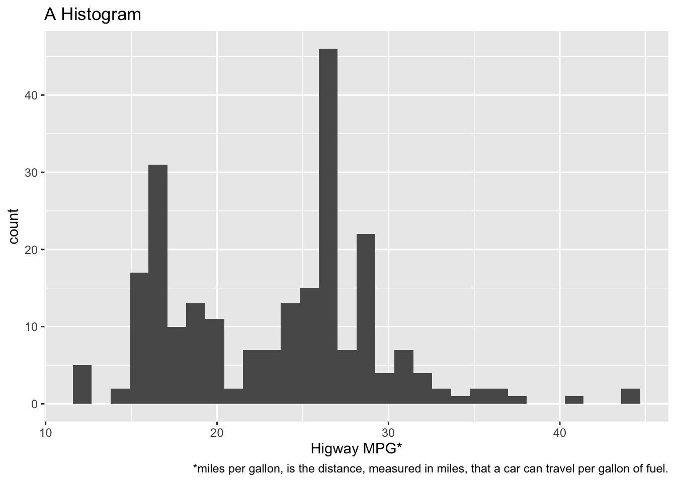
A plot on the distance that cars can travel per gallon. Note that we will hide the code when rendering by setting echo: false.
`stat_bin()` using `bins = 30`. Pick better value with `binwidth`.