Problem set 4

Author

Put your name here

# load packages
library(tidyverse)

── Attaching core tidyverse packages ──────────────────────── tidyverse 2.0.0 ──
✔ dplyr     1.1.4     ✔ readr     2.1.5
✔ forcats   1.0.0     ✔ stringr   1.5.1
✔ ggplot2   3.5.1     ✔ tibble    3.2.1
✔ lubridate 1.9.3     ✔ tidyr     1.3.1
✔ purrr     1.0.2     
── Conflicts ────────────────────────────────────────── tidyverse_conflicts() ──
✖ dplyr::filter() masks stats::filter()
✖ dplyr::lag()    masks stats::lag()
ℹ Use the conflicted package (<http://conflicted.r-lib.org/>) to force all conflicts to become errors

set.seed(1234) # For reproducibility

Read the survey data.

# Load the survey data from class
survey <- read_csv("../data/distance-to-school_pet-preferences.csv")

In this solution, we’ll use simulated data.

# simulate survey data
sample_size <- 30

survey <- tibble(
  name = 1:sample_size,
  distance = round(runif(sample_size, min = 0.3, max = 20), 1),
  pet_preference = sample(c("dogs", "cats"), size = sample_size, replace = TRUE)
)

Step 1: Calculate an estimate based on your sample

# compute rating difference in the sample
survey_estimate <- survey |> 
  group_by(pet_preference) |> 
  summarize(avg_distance = mean(distance)) |> 
  summarise(diff = avg_distance[pet_preference == "dogs"] - avg_distance[pet_preference == "cats"]) %>%
  pull(diff)

survey_estimate

[1] -0.6533333

In our sample, cat people live further away, on average.

Step 2: Use simulation to invent a world where the true effect is null.

Simulate a population, say all students in Paris, i.e. 700’000 students.

# simulate survey data
population_size <- 700000

population <- tibble(
  name = 1:population_size,
  distance = round(runif(population_size, min = 0.3, max = 20), 1),
  pet_preference = sample(c("dogs", "cats"), size = population_size, replace = TRUE)
)

Simulate 1000 samples with the same sample size that your estimate is based on. Store the estimates of this simulation in a vector called sampling_distribution.

n_simulations <- 1000
sample_size <- 30
differences <- c() # make an empty vector

for (i in 1:n_simulations) {
  # draw a sample of 20'000 films
  sample <- population |> 
    sample_n(sample_size)
  # compute rating difference in the sample
  estimate <- sample |> 
    group_by(pet_preference) |> 
    summarize(avg_distance = mean(distance)) |> 
    summarise(diff = avg_distance[pet_preference == "dogs"] - avg_distance[pet_preference == "cats"]) %>%
    pull(diff)
  
  differences[i] <- estimate
}

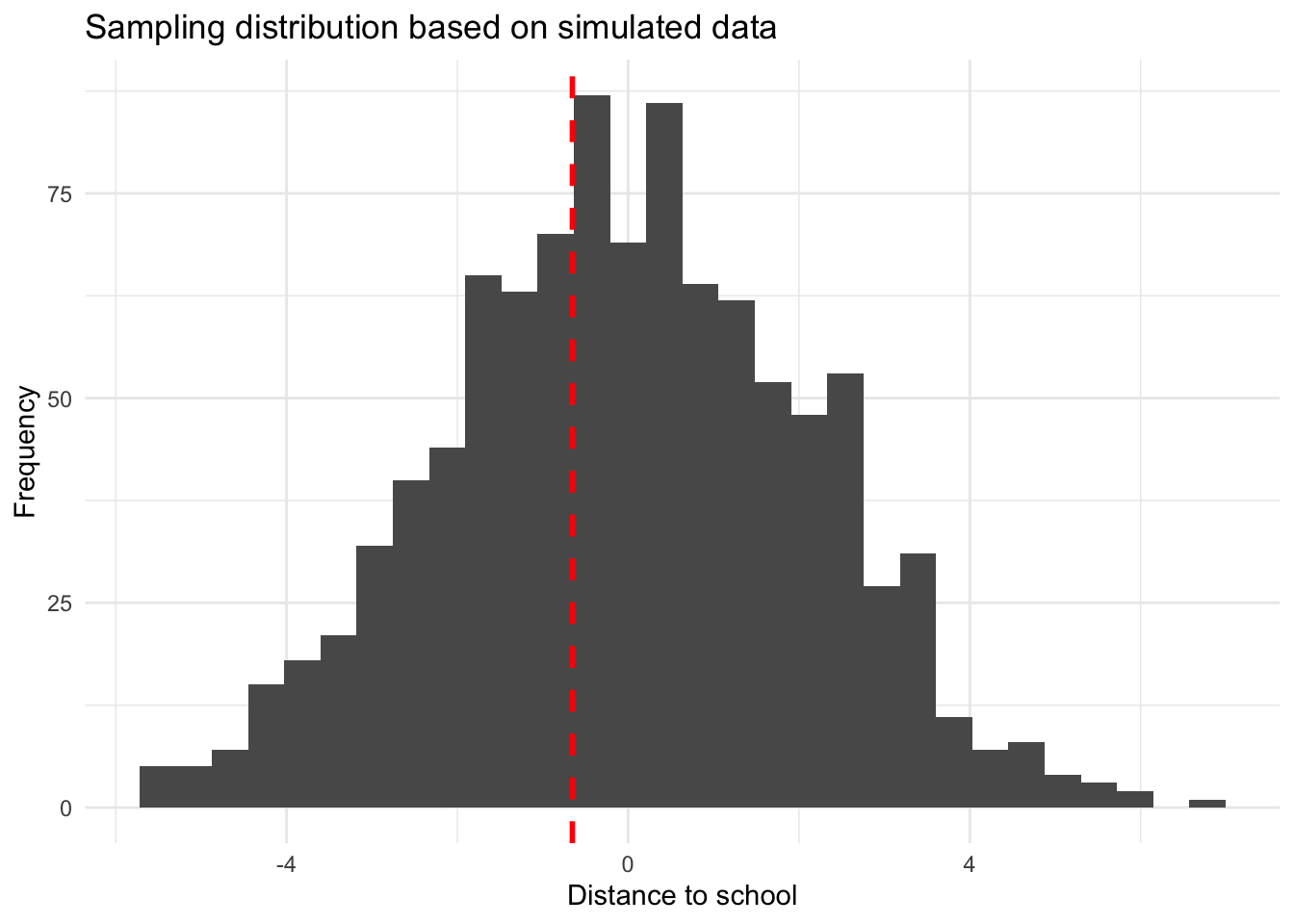
Step 3: Plot how well this estimate fits into your null world.

ggplot(data.frame(differences), aes(x = differences)) +
  geom_histogram() +
  geom_vline(xintercept = survey_estimate, color = "red", size = 1, linetype = "dashed") +
  labs(title = "Sampling distribution based on simulated data",
       x = "Distance to school",
       y = "Frequency") +
  theme_minimal()

Warning: Using `size` aesthetic for lines was deprecated in ggplot2 3.4.0.
ℹ Please use `linewidth` instead.

`stat_bin()` using `bins = 30`. Pick better value with `binwidth`.

Step 4: Calculate the probability that your estimate could exist in the null world.

Use the standard deviation of your sampling_distribution to transform your initial estimate in a z-value.

sd_sampling_distribution <- sd(differences)

z_scaled_estimate = survey_estimate / sd_sampling_distribution

z_scaled_estimate

[1] -0.3074499

Based on this, calculate the p-value.

# the pnorm() function gives the cumulative probability from the standard normal distribution 

# Two-tailed (i.e. a value "at least as extreme as", in both directions)
probability <- 2 * (1 - pnorm(z_scaled_estimate)) 

# in our case, the probability is reeaally low (practically 0)
probability

[1] 1.241499

Step 5: Decide if your estimate is statistically significant.

Use a significance threshold (the value at which you consider your estimate sufficiently unlikely to have occurred in the Null World) of 0.05

# significance levels are often called "alpha"
alpha <- 0.05

probability < alpha

[1] FALSE

No, our estimate is not statistically significant: We cannot cannot reject the Null hypothesis that in fact, in the population, there is no true effect. In other words, in a world where there is no effect, it does not appear sufficiently unlikely to randomly sample an estimate at least as big as the one we found.

Is this result surprising to you or not? Explain.

This result is probably not surprising, since we would hardly expect a relationship between pet preferences and distance to school a priori.

Other Formats