── Attaching core tidyverse packages ──────────────────────── tidyverse 2.0.0 ──
✔ dplyr     1.1.4     ✔ readr     2.1.5
✔ forcats   1.0.0     ✔ stringr   1.5.1
✔ ggplot2   3.5.1     ✔ tibble    3.2.1
✔ lubridate 1.9.3     ✔ tidyr     1.3.1
✔ purrr     1.0.2
── Conflicts ────────────────────────────────────────── tidyverse_conflicts() ──
✖ dplyr::filter() masks stats::filter()
✖ dplyr::lag()    masks stats::lag()
ℹ Use the conflicted package (<http://conflicted.r-lib.org/>) to force all conflicts to become errors
library(broom)
Read the survey data.
# Load the survey data from classpenguins <-read_csv("../data/penguins.csv")
Rows: 342 Columns: 8
── Column specification ────────────────────────────────────────────────────────
Delimiter: ","
chr (3): species, island, sex
dbl (5): bill_length_mm, bill_depth_mm, flipper_length_mm, body_mass_g, year

ℹ Use `spec()` to retrieve the full column specification for this data.
ℹ Specify the column types or set `show_col_types = FALSE` to quiet this message.
Graphs
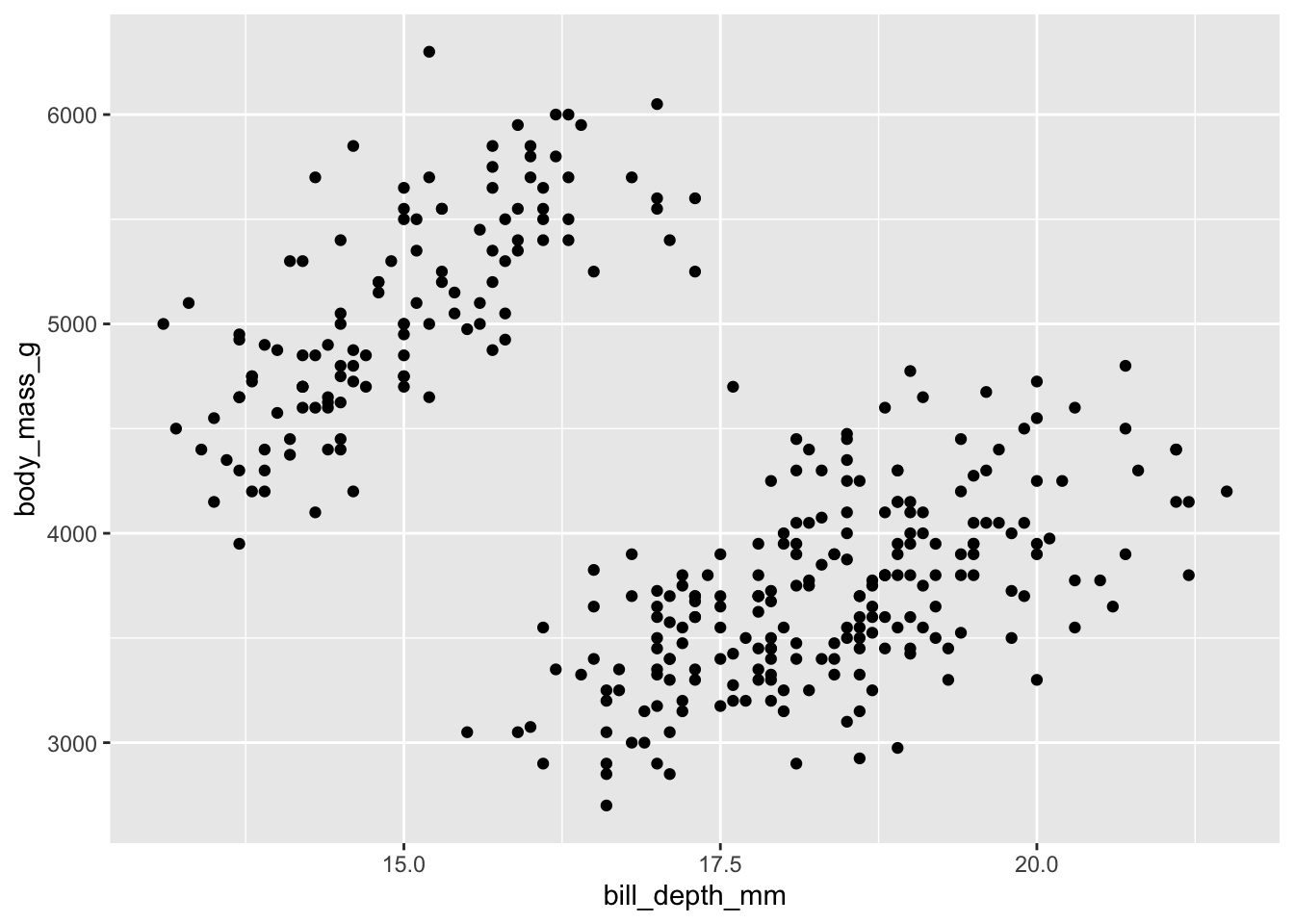
What is the relationship between penguin weight and bill depth? This plot shows some initial trends:
ggplot(data = penguins, aes(x = bill_depth_mm, y = body_mass_g)) +geom_point()
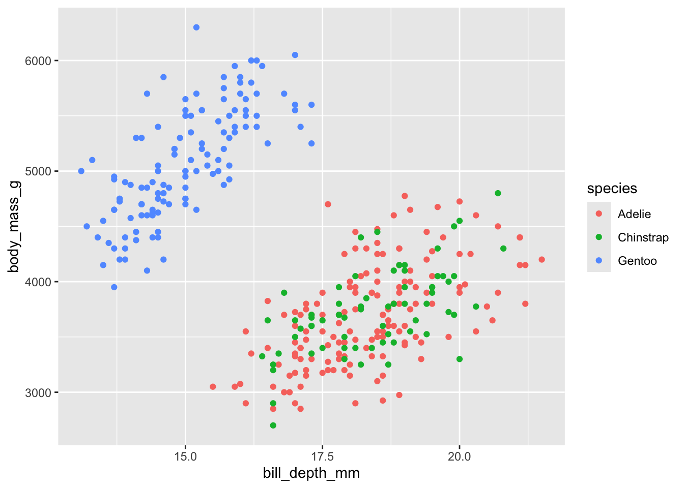
Make a new plot that colors these points by species. What can you tell about the relationship between bill depth and penguin weight?
ggplot(data = penguins, aes(x = bill_depth_mm, y = body_mass_g, color = species)) +geom_point()
It seems like the longer the bill, the greater the body mass, but only within species. If we ignore the species it looks like greater bill depth is associated with lower body mass.
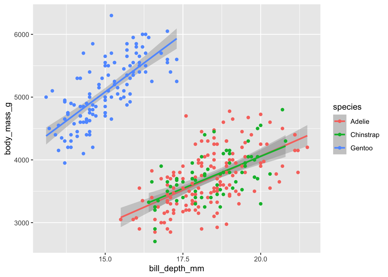
Add a geom_smooth() layer to the plot and make sure it uses a straight line (hint: include method="lm" in the function). What does this tell you about the relationship between bill depth and body mass?
ggplot(data = penguins, aes(x = bill_depth_mm, y = body_mass_g, color = species)) +geom_smooth(method ="lm") +geom_point()
`geom_smooth()` using formula = 'y ~ x'
This confirms that within different species, there is a positive relationship.
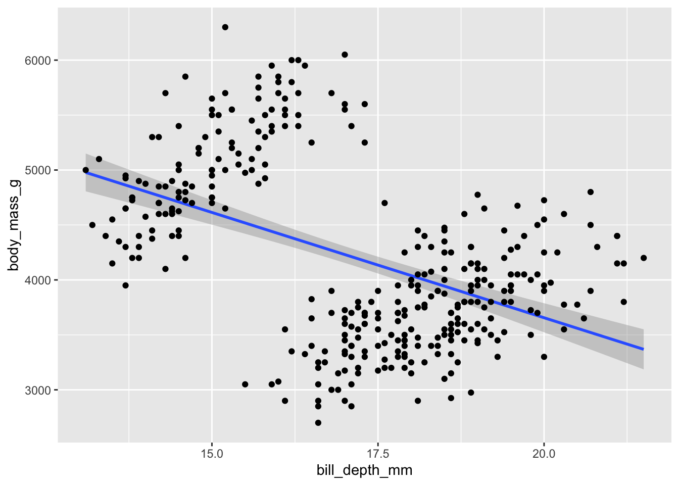
Change the plot so that there’s a single line for all the points instead of one line per species. How does the slope of this single line differ from the slopes of the species specific lines? Why??
By removing the color layer, geom_smooth only draws one line considering all of the data. Glancing over species, there is actually a negative association between bill depth and body mass in the data.
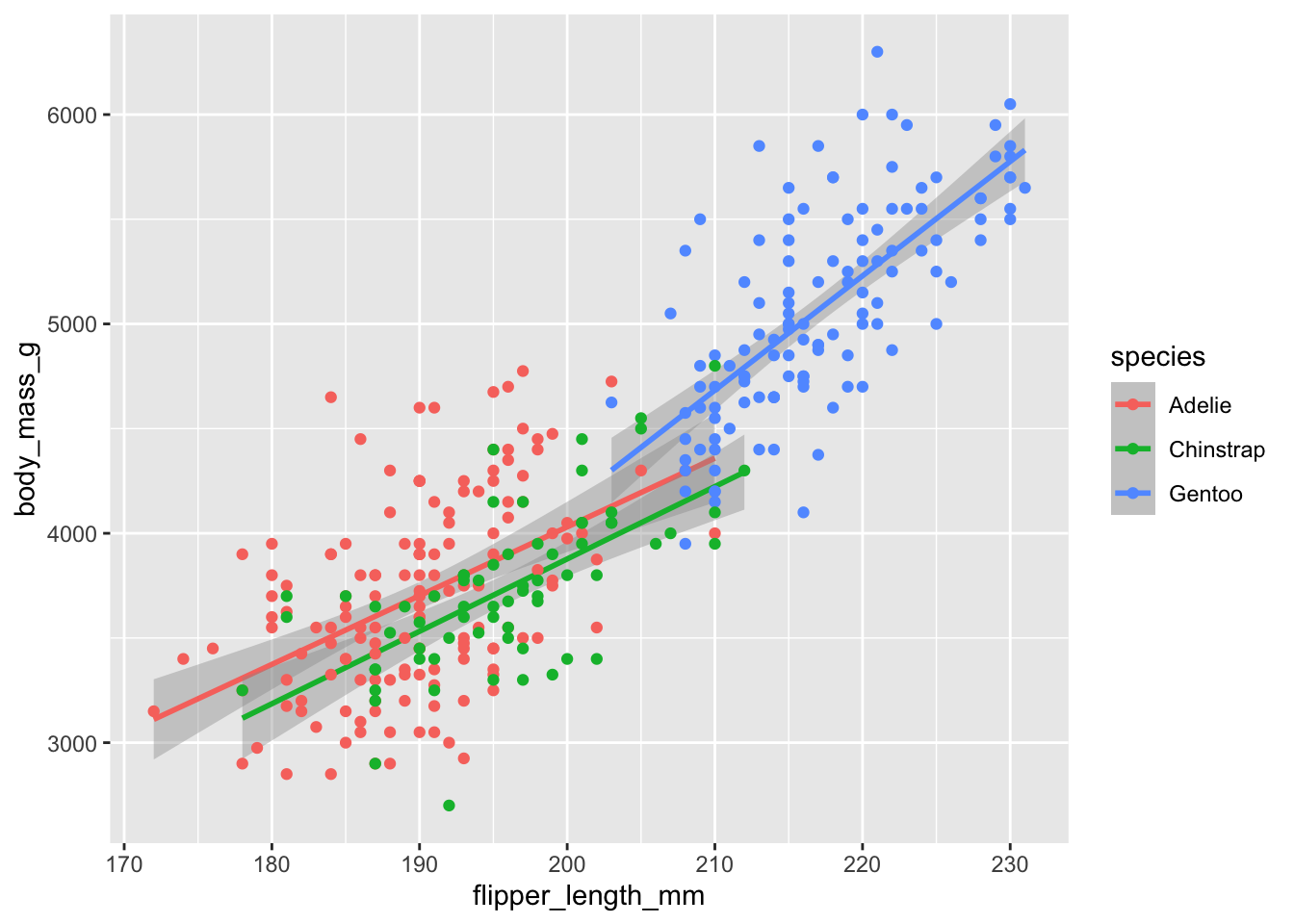
What is the relationship between flipper length and body mass? Make another plot with flipper_length_mm on the x-axis, body_mass_g on the y-axis, and points colored by species.
ggplot(data = penguins, aes(x = flipper_length_mm, y = body_mass_g, color = species)) +geom_smooth(method ="lm") +geom_point()
`geom_smooth()` using formula = 'y ~ x'
There is a positive relationship between flipper length and body mass, both within and across species.
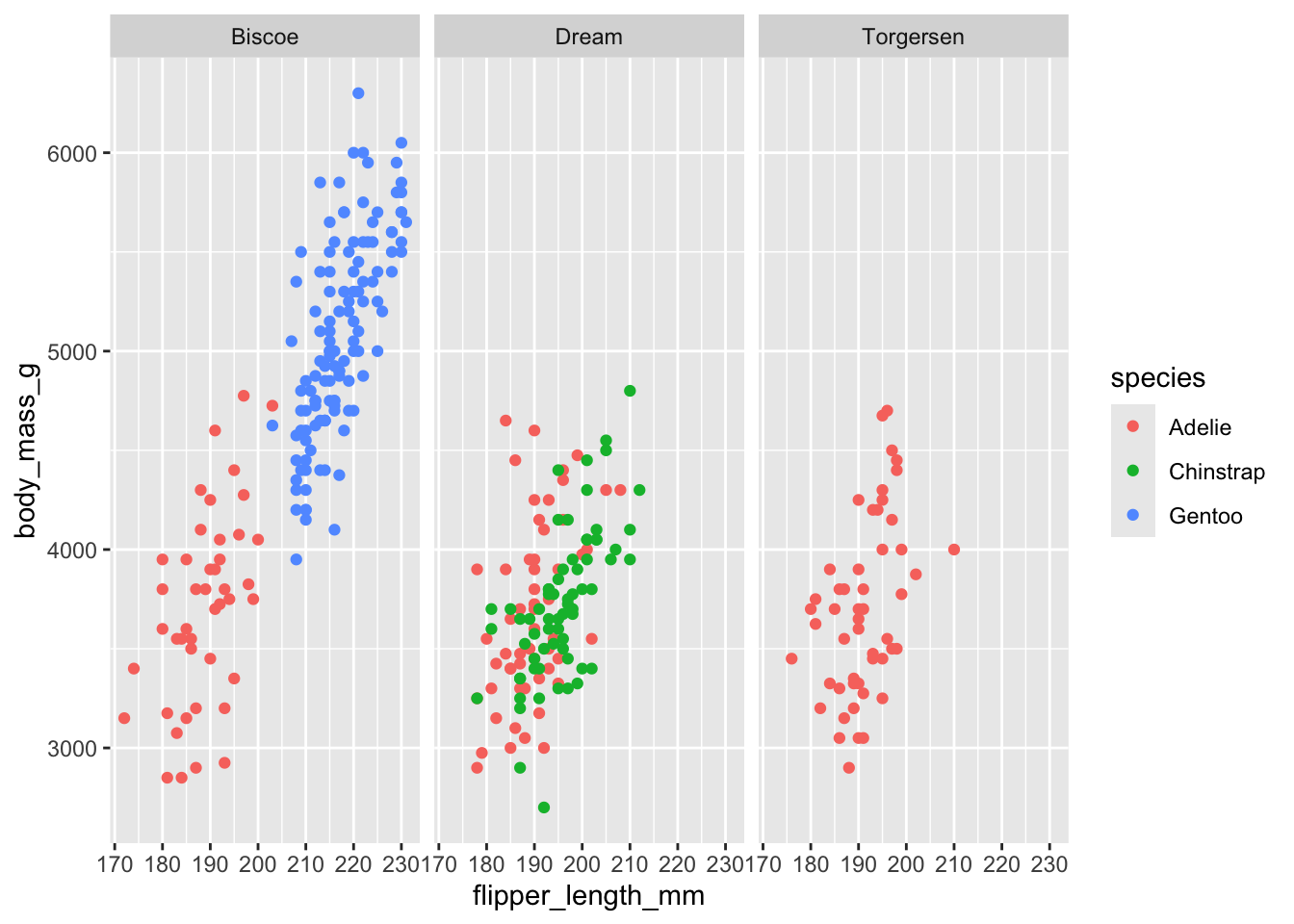
Facet (facet_wrap) the plot by island (island). What does this graph tell you ?
ggplot(data = penguins,aes(x = flipper_length_mm, y = body_mass_g, color = species)) +geom_point() +facet_wrap(vars(island))
There is a positive relationship between flipper length and body mass, for all species. However, not all species are present on all islands. Of the Gentoo, the penguins with the smalles flipper length still have flipper lengths of the size as the biggest once of the Chinstrap and Adelie.
Regression
Does bill depth predict penguin weight? Run a linear regression (lm()) and interpret the estimate and the p.value. Interpret the result in light of previous plots that you have generated.
Yes, bill depth does predict penguin weight, negatively. A one mm increase in bill depth is associated with approximately 191 gramms less body weight. However, as we saw earlier in the plots, this is only true when comparing across species. Within species the opposite is true. This result is statistically significant, as indicated by the low p-value (smaller than 0.05).
Run different regression analyses for the different species (use filter()) to subset the data frame.
# check different speciestable(penguins$species)
   Adelie Chinstrap    Gentoo
      151        68       123
regression_adelie <-lm(body_mass_g ~ bill_depth_mm, data = penguins |>filter(species =="Adelie")) regression_chinstrap <-lm(body_mass_g ~ bill_depth_mm, data = penguins |>filter(species =="Chinstrap"))regression_gentoo <-lm(body_mass_g ~ bill_depth_mm, data = penguins |>filter(species =="Gentoo"))# we can use the modelsummary package to display the results of all three regressions at oncemodelsummary::modelsummary(list("Adelie"= regression_adelie, "Chinstrap"= regression_chinstrap, "Gentoo"= regression_gentoo), statistic ="p.value", stars =TRUE)
Adelie
Chinstrap
Gentoo
+ p < 0.1, * p < 0.05, ** p < 0.01, *** p < 0.001
(Intercept)
-283.279
-36.219
-458.985
(0.542)
(0.953)
(0.348)
bill_depth_mm
217.152***
204.625***
369.441***
(<0.001)
(<0.001)
(<0.001)
Num.Obs.
151
68
123
R2
0.332
0.365
0.517
R2 Adj.
0.327
0.356
0.513
AIC
2223.3
976.4
1795.3
BIC
2232.3
983.1
1803.8
Log.Lik.
-1108.647
-485.224
-894.666
RMSE
373.57
303.90
348.89
As observered earlier in the plots, we find a positive association between bill depth and body mass for all species when analyzed seperately. These results are statistically significant, as indicated by the low p-values (smaller than 0.05).