| Category | Description | Notation |
|---|---|---|
| Data | IMDB ratings | \(D\) |
| Calculation | Average action rating − average comedy rating | \(\bar{D} = \frac{\sum{D}_\text{Action}}{N} - \frac{\sum{D}_\text{Comedy}}{N}\) |
| Estimate | \(\bar{D}\) in a sample of movies | \(\hat{\delta}\) |
| Truth | Difference in rating for all movies | \(\delta\) |
Statistical Inference
Simulated Null World
Our simulated action movies and comedies don’t all have the same rating, but on average there’s (almost) no difference
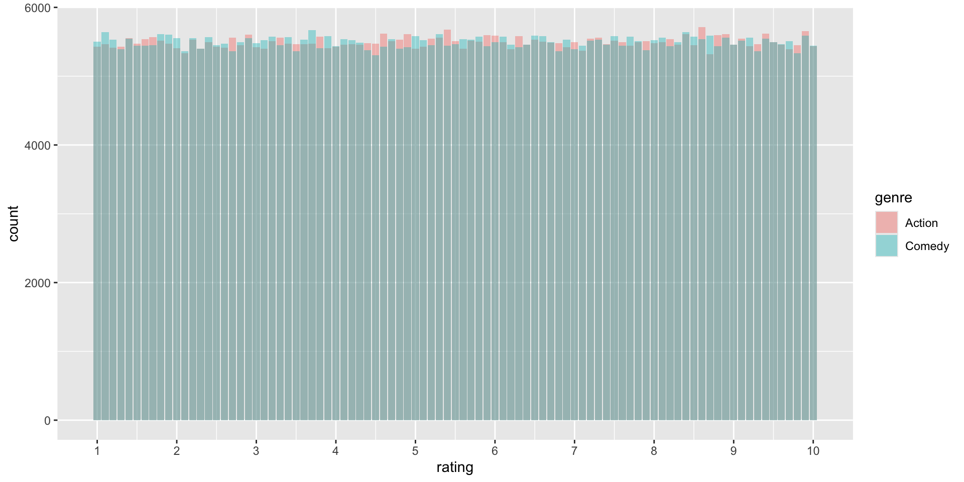
We can plot the results for an overview
n_simulations <- 1000
differences <- c() # make an empty vector
for (i in 1:n_simulations) {
# draw a sample of 20'000 films
imaginary_sample <- imaginary_movies |>
  sample_n(20000)
# compute rating difference in the sample
estimate <- imaginary_sample |>
group_by(genre) |>
summarize(avg_rating = mean(rating)) |>
summarise(diff = avg_rating[genre == "Action"] - avg_rating[genre == "Comedy"]) %>%
pull(diff)
differences[i] <- estimate
}
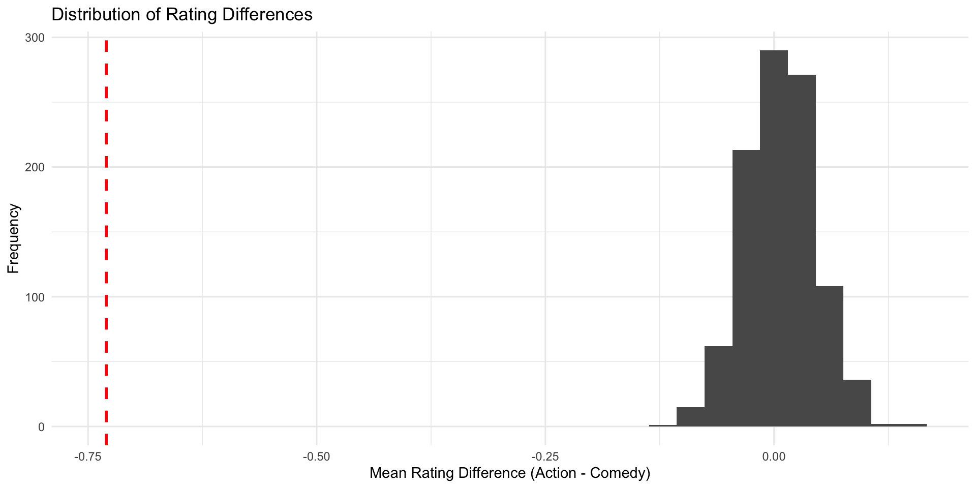
Check \(\hat{\delta}\) in the null world
Does the estimate we found in the IMDB data (\(\hat{\delta}\) = -0.73) fit well into the world where the true difference \(\delta\) is 0?

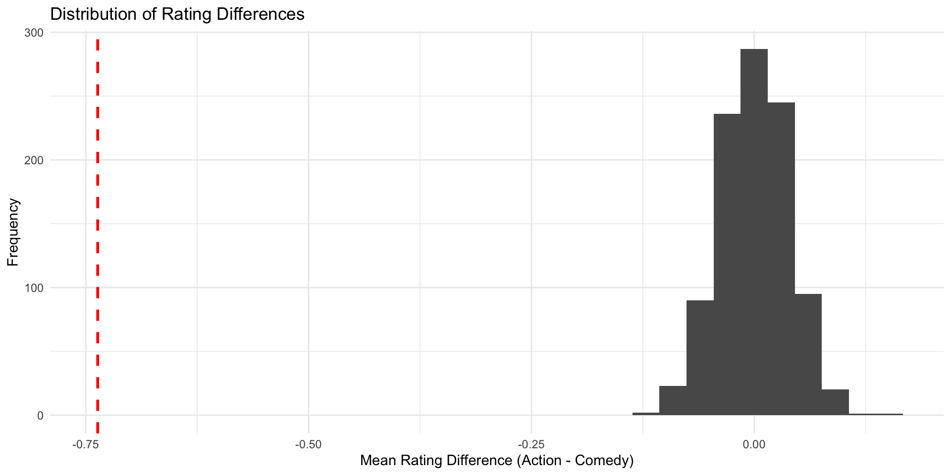
Check \(\hat{\delta}\) in the null world
Does the estimate we found in the IMDB data (\(\hat{\delta}\) = -0.73) fit well into the world where the true difference \(\delta\) is 0? Not really.

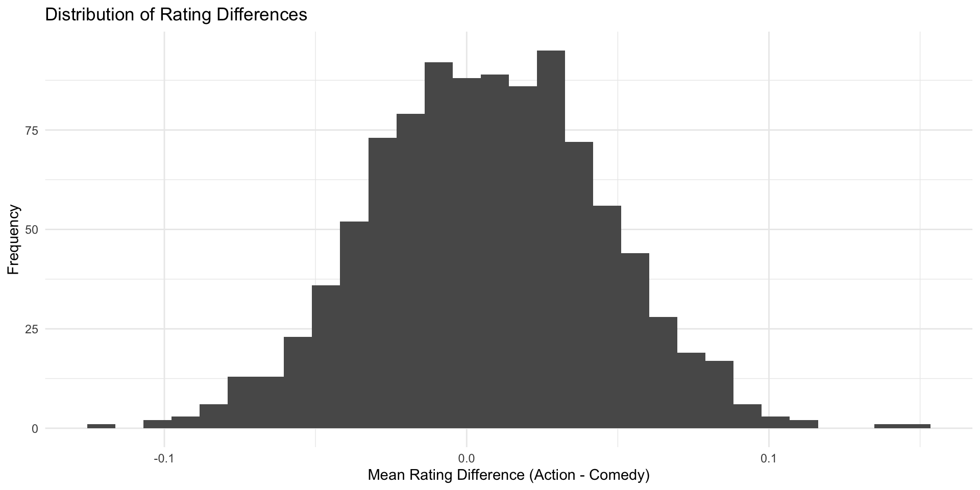
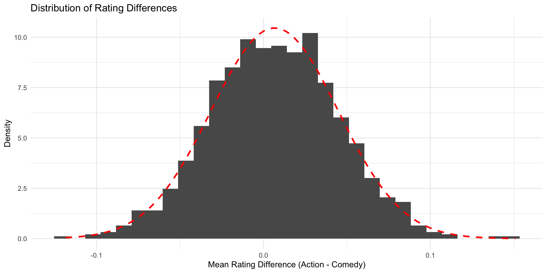
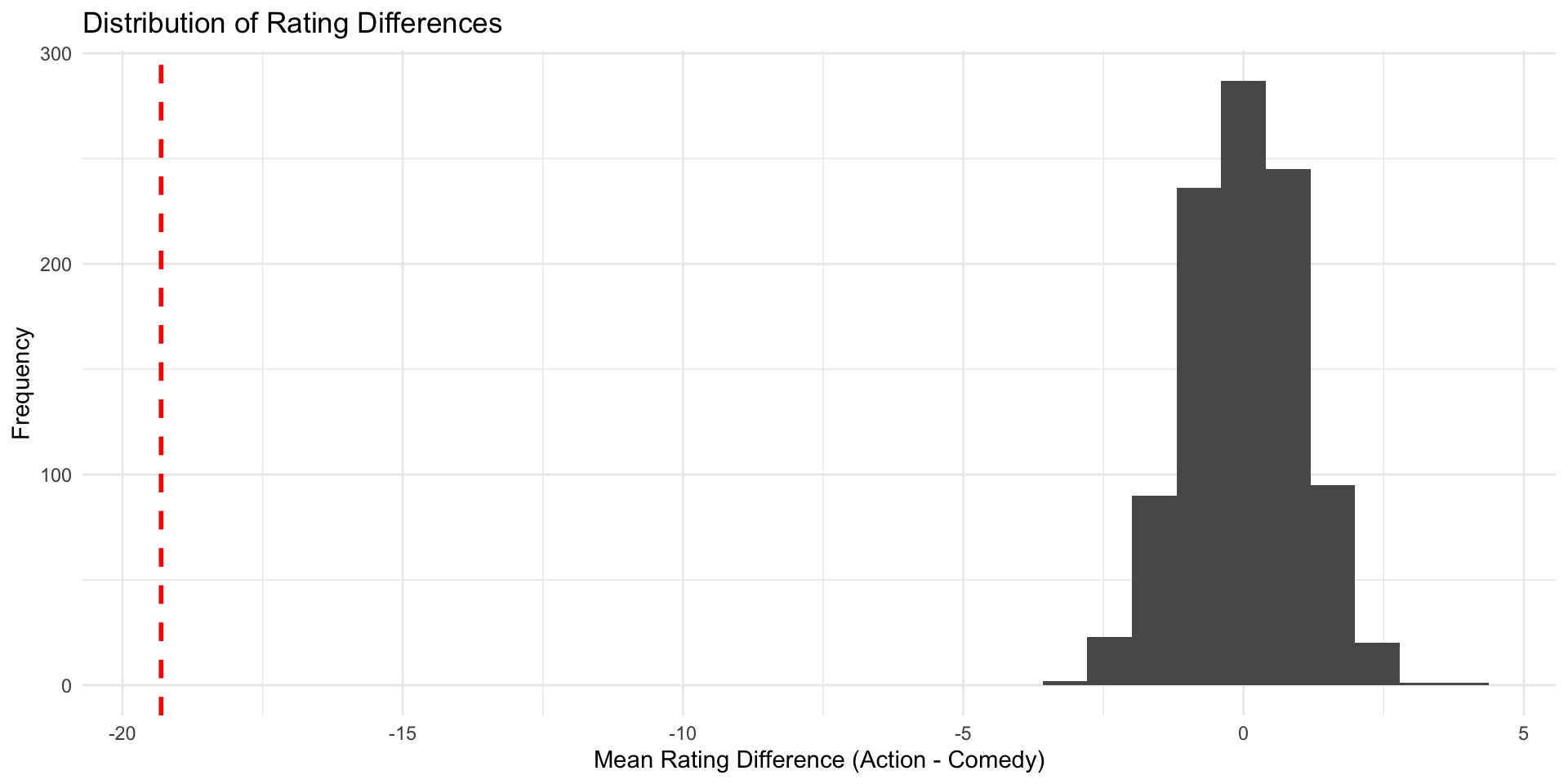
You have seen before the estimated mean differences of our imaginary samples (the \(\hat{\delta}s\)), somehow magically, form a curve that is…
- bell-shaped
- centered around the true value (\(\delta\)), which in our case was 0.
This distribution of estimates is also called the sampling distribution.
The central limit theorem states that, with many observations, the sampling distribution approximates a normal distribution.
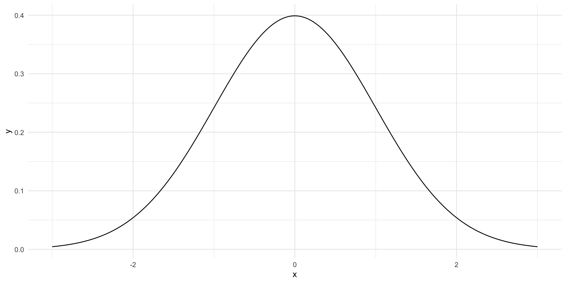
The most famous bell-shaped distribution is the (standard) normal distribution.
The standard normal distribution is centered around 0 and has a standard deviation of 1.
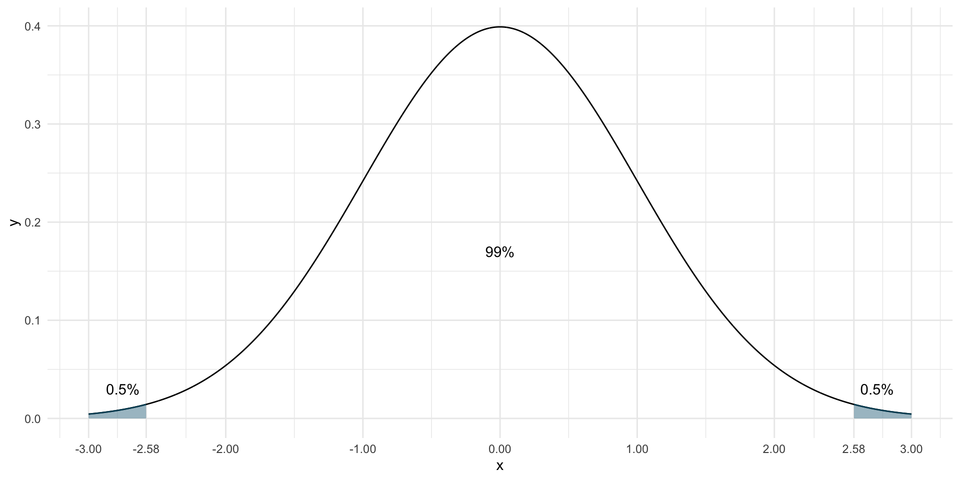
We know, e.g., that 99% of the distribution lie between \(\pm\) 2.58
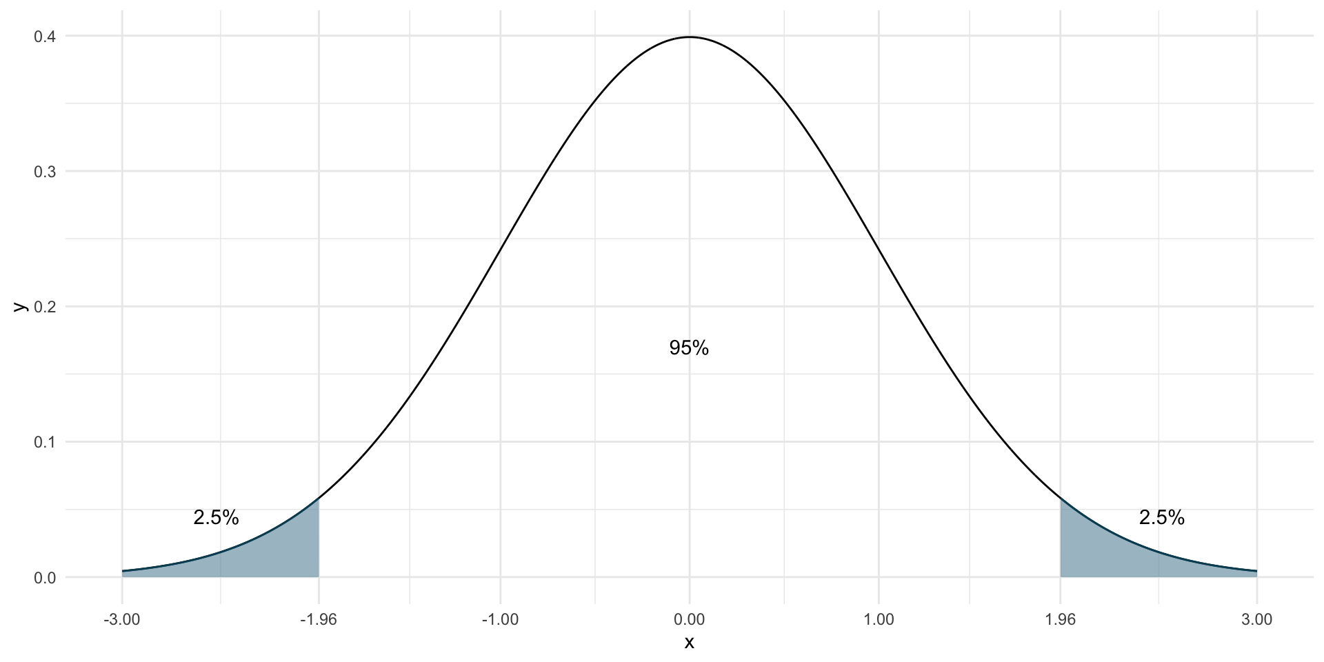
Or that 95% of the distribution lie between \(\pm\) 1.96
Now, all we need to do is bring our sampling distribution on the scale of a standard normal distribution.
Now, all we need to do is bring our sampling distribution on the scale of a standard normal distribution.
We achieve this by
- Subtracting the mean from all values (in our case, that is 0, so nothing happens)
In our case, that is (almost) 0, so not much happens

Now, all we need to do is bring our sampling distribution on the scale of a standard normal distribution.
We achieve this by
Subtracting the mean from all values
Dividing by the standard deviation
Since the sd is small than 1, our values become bigger

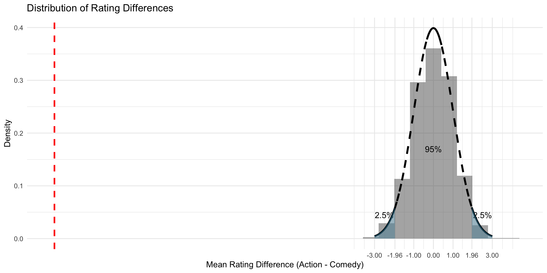
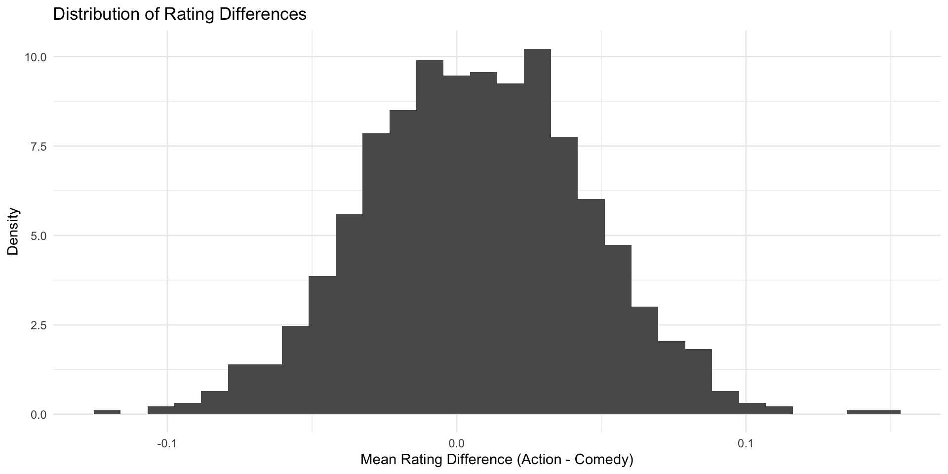
Instead of a histogram, we can use a density plot (which uses the same y-axis as the normal distribution, namely density)


Finally, we can lay over the standard normal distribution
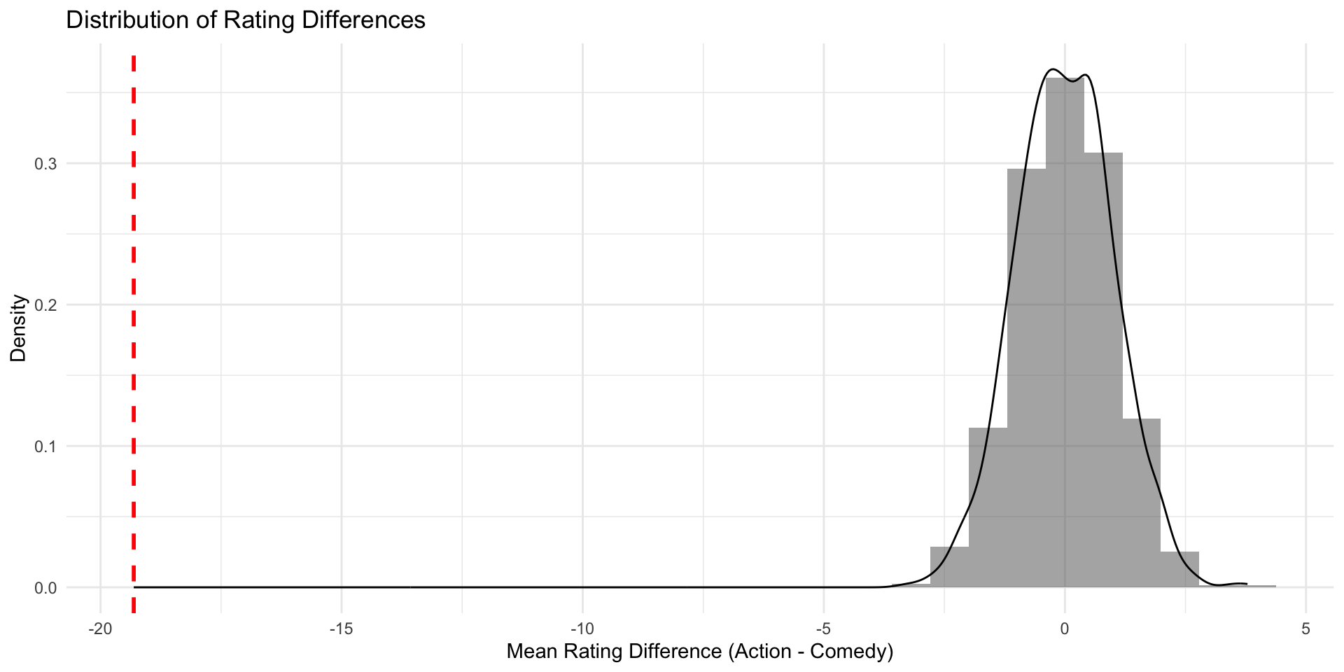
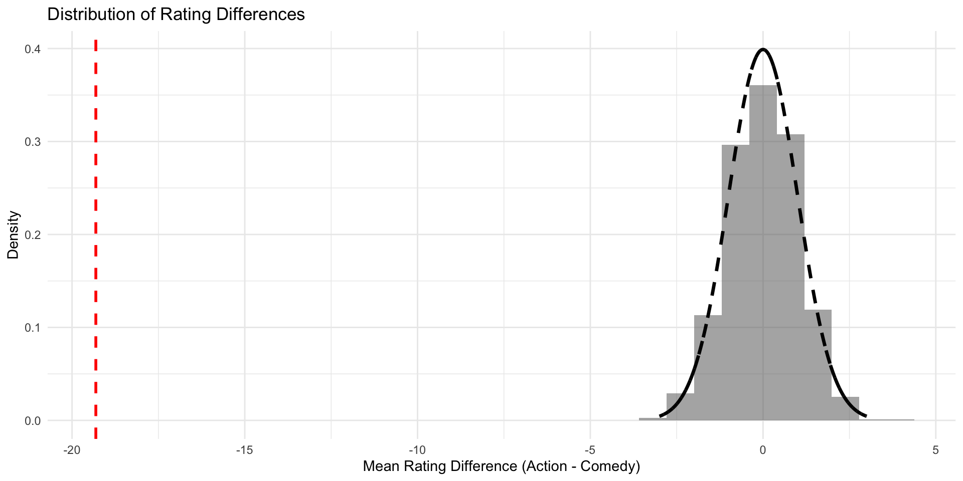
Now we can say for sure that in our Null world, chances that we get an estimate as extreme as the one in our IMBD data is less than 5%