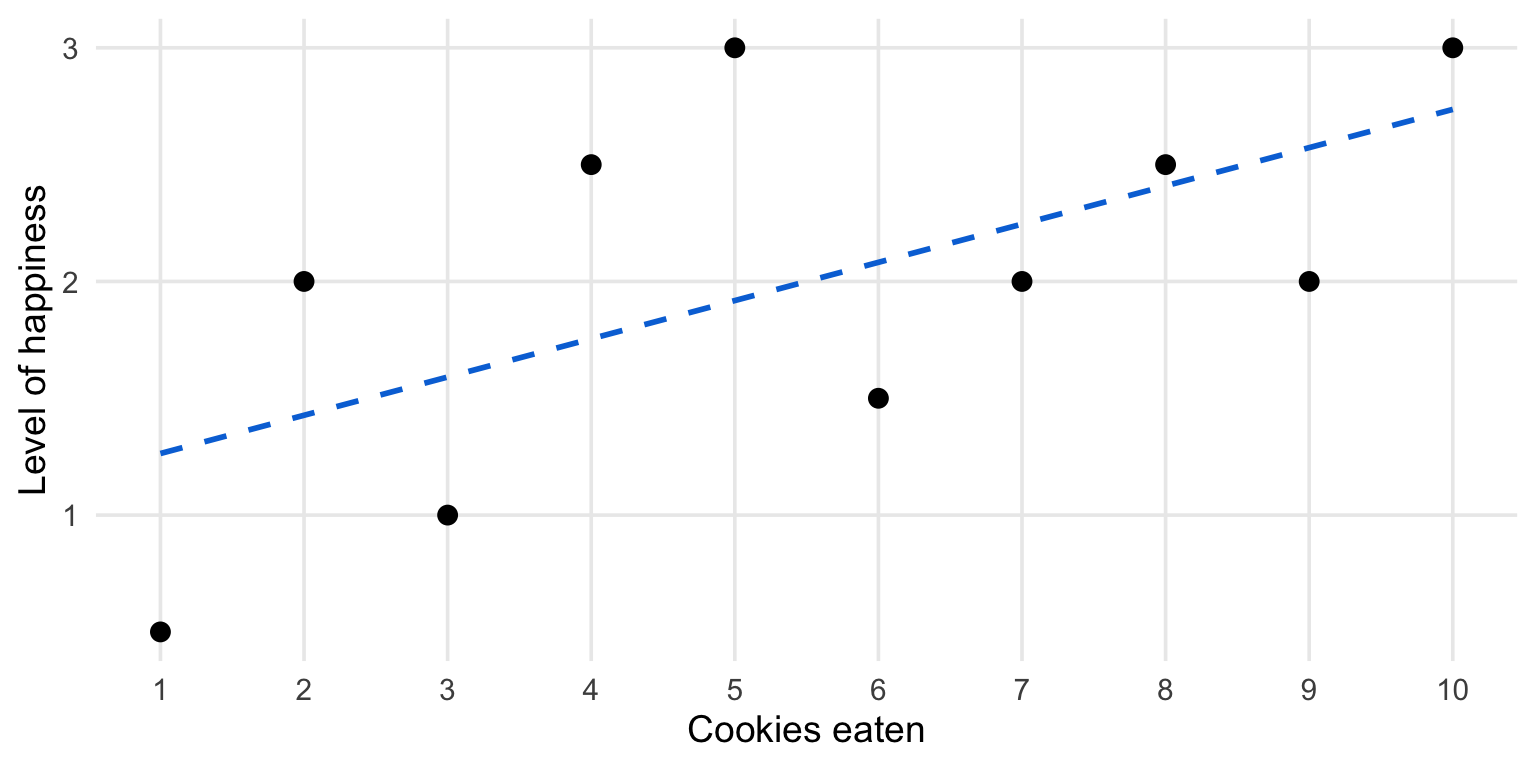
Linear Regression
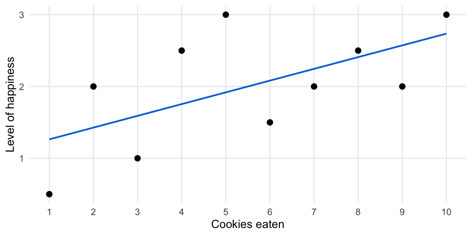
Cookies and happiness
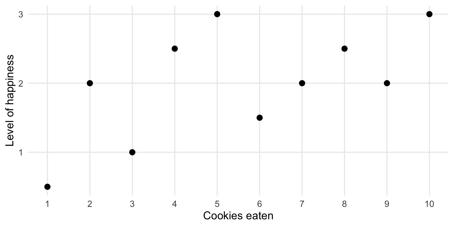
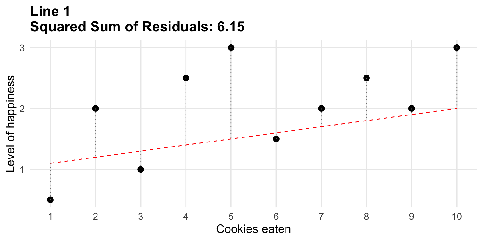
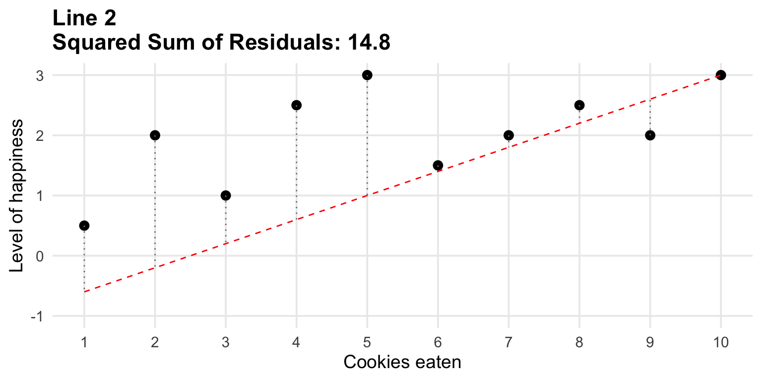
How good is the fit?
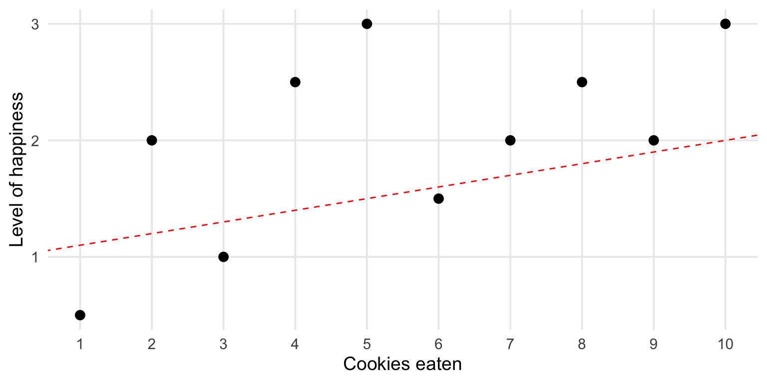
How good is the fit?
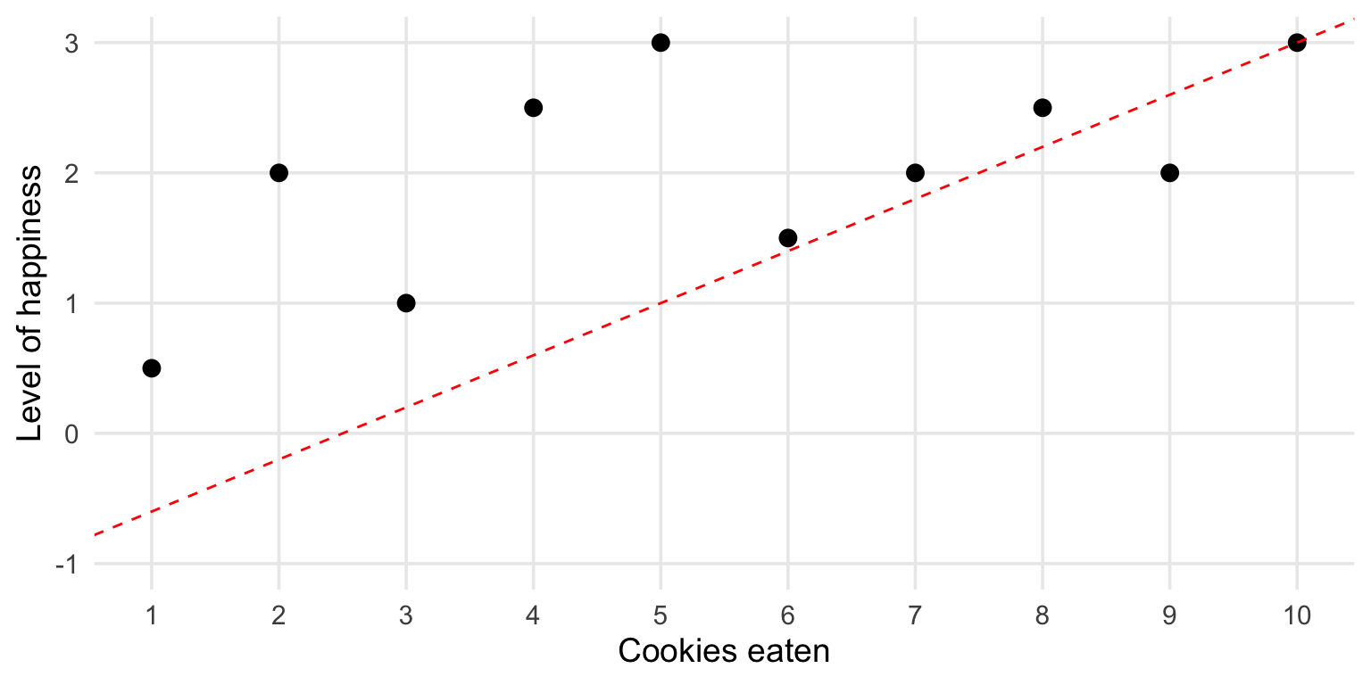
How good is the fit?
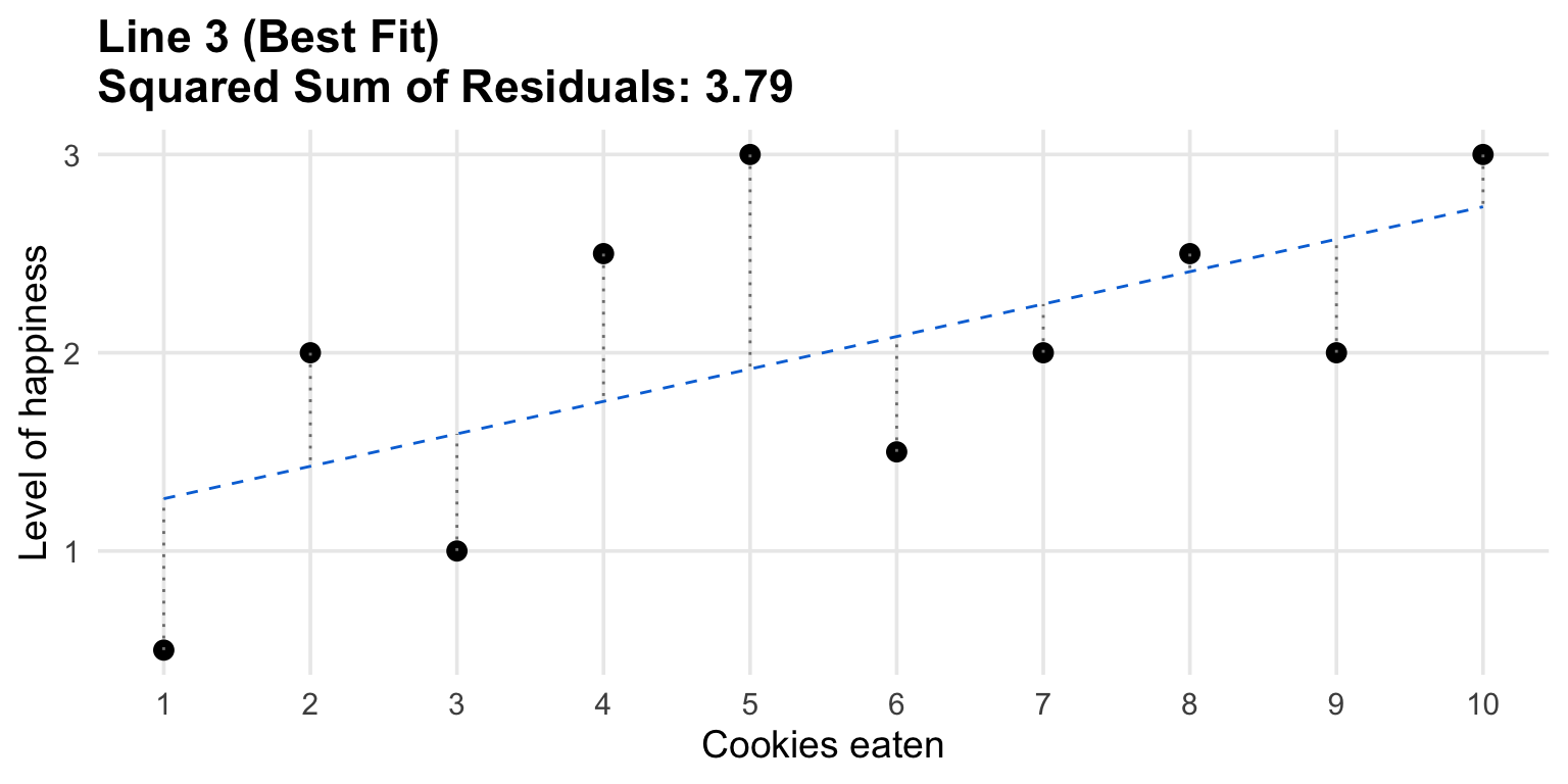
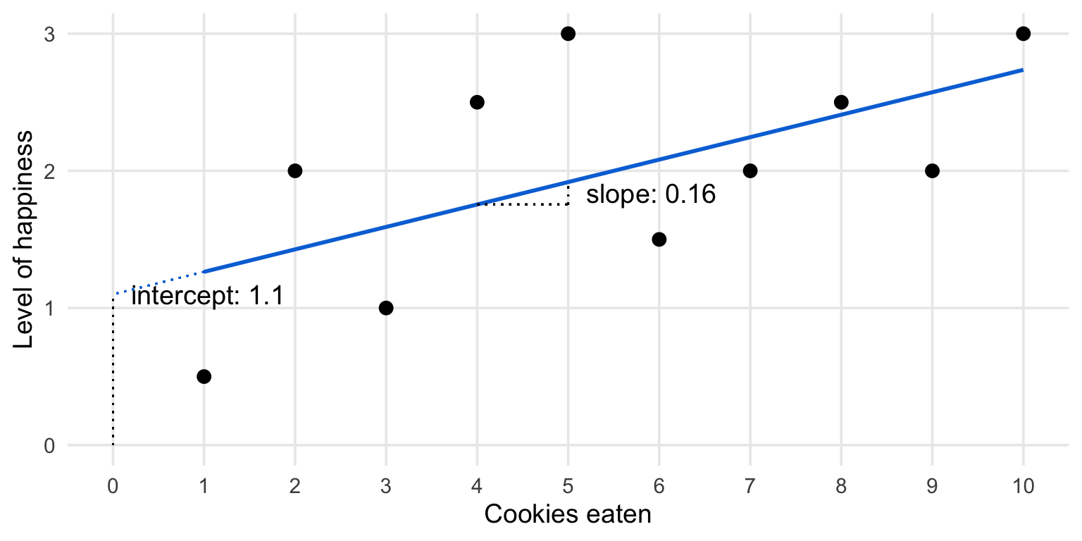
Linear regression estimates
Linear regression estimates
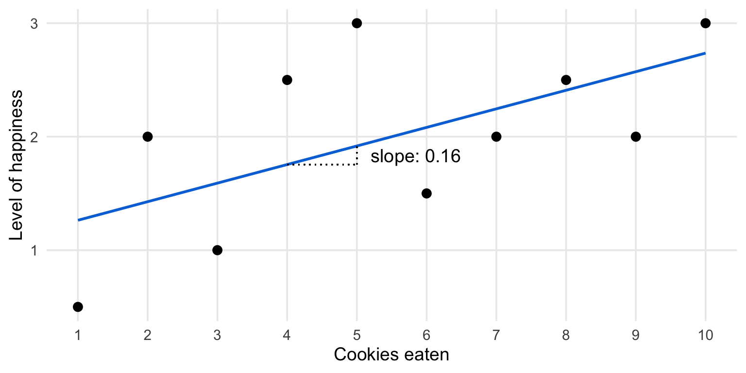
Linear regression estimates
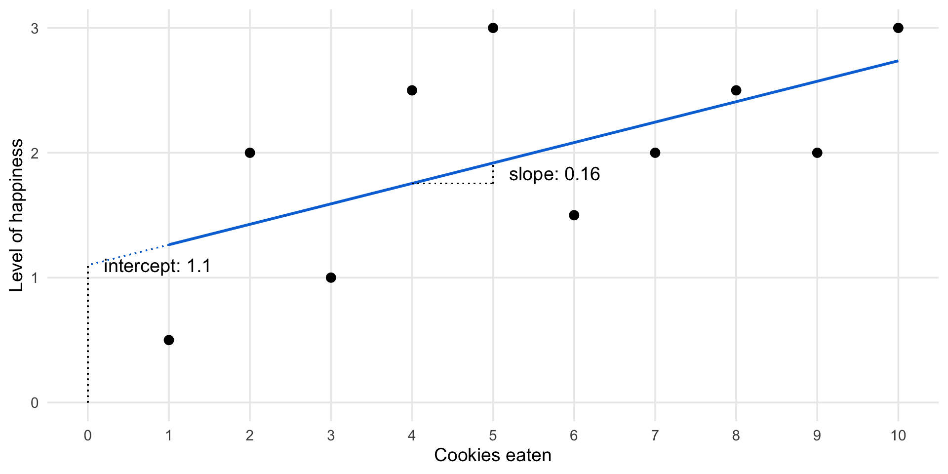
Interpreting linear regression output
“A one unit increase in X is associated with a beta 1 increase (or decrease) in Y, on average.”
We get some more detail doing this:
# Compute the OLS regression model
ols_model <- lm(happiness ~ cookies, data = cookies)

summary(ols_model)
Call:
lm(formula = happiness ~ cookies, data = cookies)

Residuals:
     Min       1Q   Median       3Q      Max
-0.76364 -0.57955 -0.07727  0.49545  1.08182

Coefficients:
            Estimate Std. Error t value Pr(>|t|)
(Intercept)  1.10000    0.47025   2.339   0.0475 *
cookies      0.16364    0.07579   2.159   0.0629 .
---
Signif. codes:  0 '***' 0.001 '**' 0.01 '*' 0.05 '.' 0.1 ' ' 1

Residual standard error: 0.6884 on 8 degrees of freedom
Multiple R-squared:  0.3682,    Adjusted R-squared:  0.2892
F-statistic: 4.662 on 1 and 8 DF,  p-value: 0.06287
Interpreting linear regression output
“A one unit increase in X is associated with a beta 1 increase (or decrease) in Y, on average.”

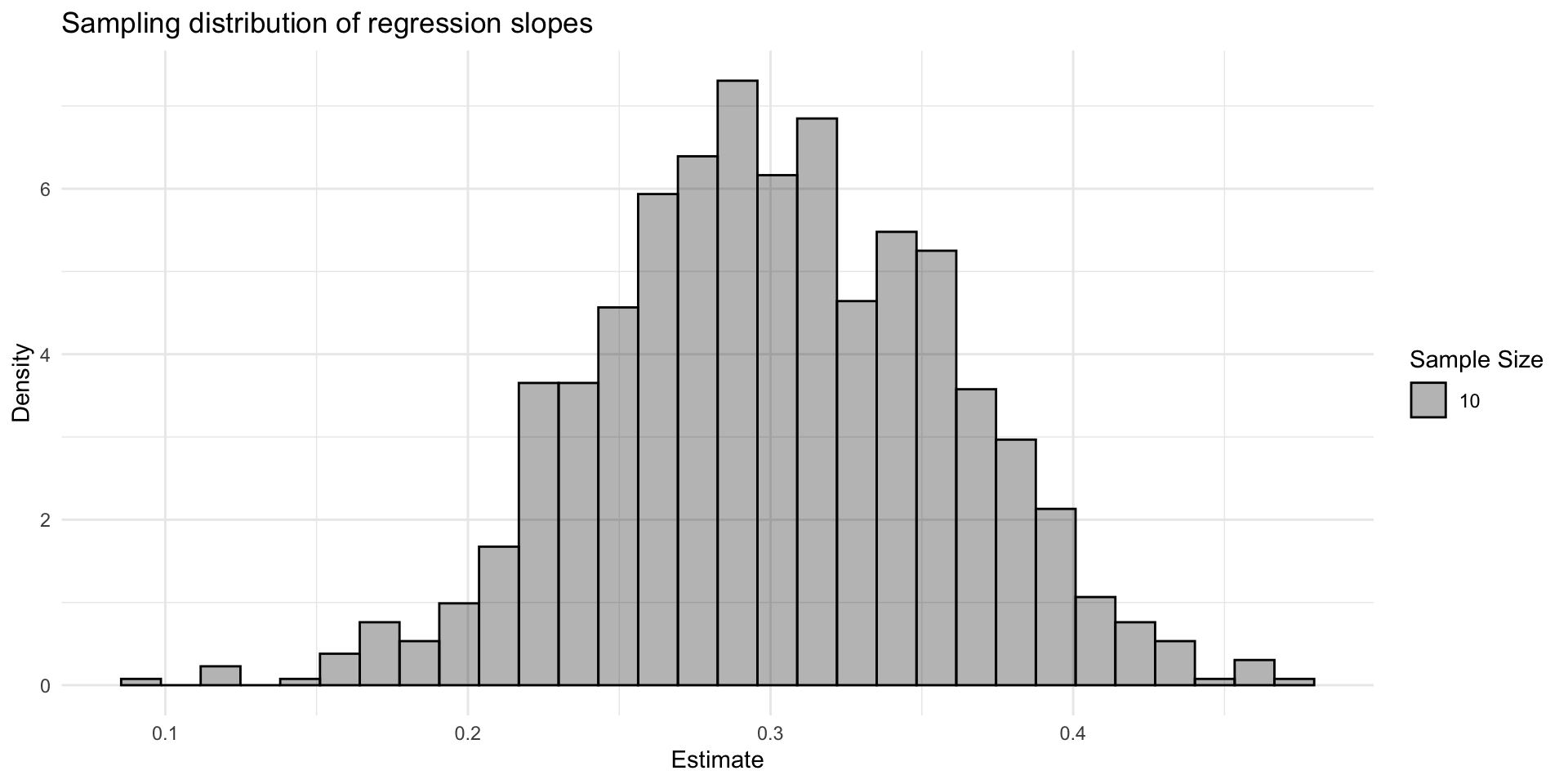
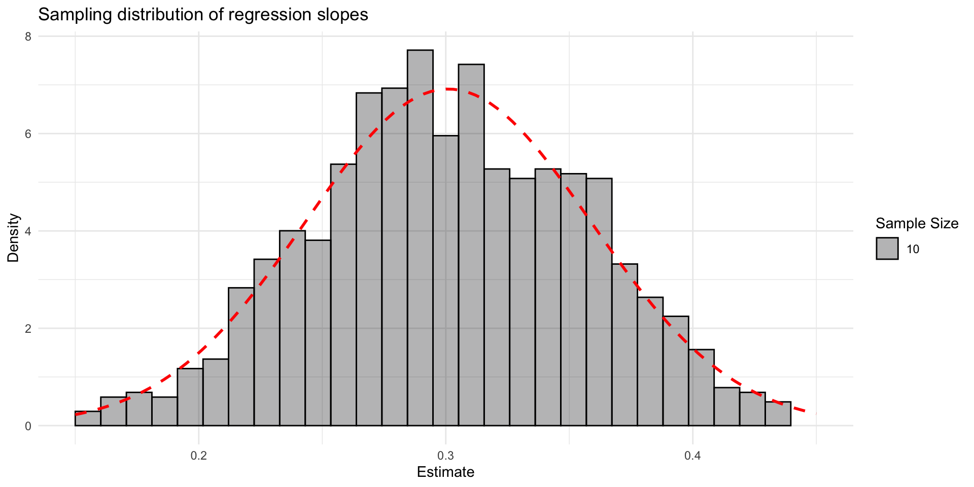
Sampling distribution
- The sampling distribution of estimates approximates a normal distribution.
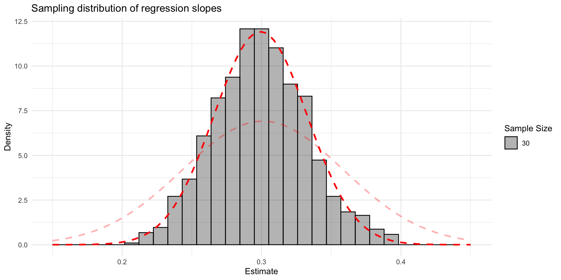
Sampling distribution
- The sampling distribution gets narrower with a larger sample size

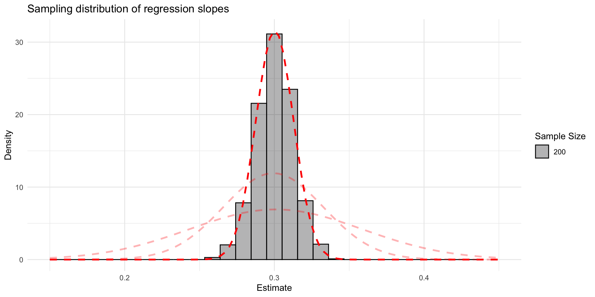
Sampling distribution
- The sampling distribution gets narrower with a larger sample size
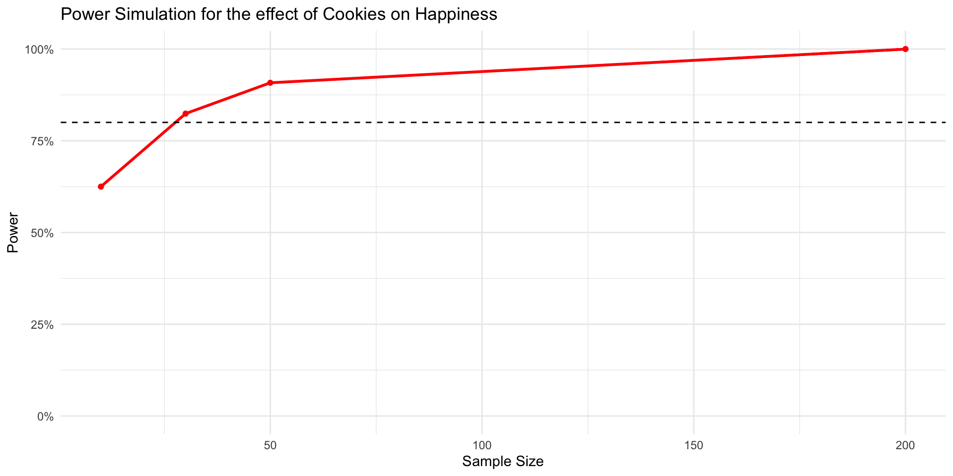
Solution
We can then plot the power curve
ggplot(power_data,
       aes(x = sample_size, y = estimated_power)) +
  geom_point(color = 'red', size = 1.5) +
  geom_line(color = 'red', size = 1) +
  # add a horizontal line at 80%
  geom_hline(aes(yintercept = .8), linetype = 'dashed') +
  # Prettify!
  theme_minimal() +
  scale_y_continuous(labels = scales::percent, limits = c(0,1)) +
  labs(title = "Power Simulation for the effect of Cookies on Happiness",
       x = 'Sample Size', y = 'Power')