Call:
lm(formula = kisses ~ self_confidence, data = kisses)

Residuals:
    Min      1Q  Median      3Q     Max
-466.55  -91.91   -0.48   80.90  437.60

Coefficients:
                Estimate Std. Error t value Pr(>|t|)
(Intercept)       99.413     35.181   2.826   0.0052 **
self_confidence   74.779      6.691  11.177   <2e-16 ***
---
Signif. codes:  0 '***' 0.001 '**' 0.01 '*' 0.05 '.' 0.1 ' ' 1

Residual standard error: 142.7 on 198 degrees of freedom
Multiple R-squared:  0.3868,    Adjusted R-squared:  0.3838
F-statistic: 124.9 on 1 and 198 DF, p-value: < 2.2e-16Colliders and Confounders
Overview
What is Causality
Correlation is not causality
Confounders
Colliders
What is Causality?
We all have an idea of what “causality” means.
Whenever we ask “why” question, we are asking for a cause.
A simple definition
We could say that X causes Y if…
we were we to intervene and change the value of X without changing anything else…
and then Y would change as a result.
Associations vs. Causality
How do we figure out associations?
Looking at data, using math and statistics
How do we figure out causation?
Philosophy (and good research design). No math or stats.
Confounders
Does self-confidence make you being kissed more often?
Imagine you are a researcher and have this (slightly stupid) research question.
What does this (made up!) data suggest?
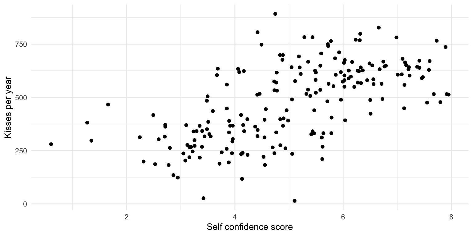
There appears to be a relationship!
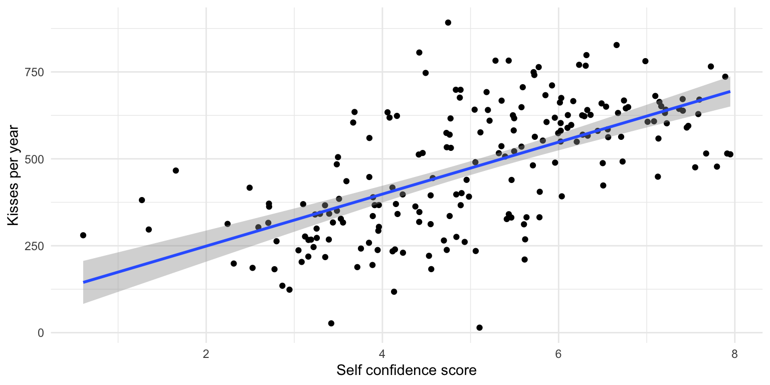
We can run the regression
🎉 We have an answer to our research question!
Or, wait, do we?
What does plot suggest?
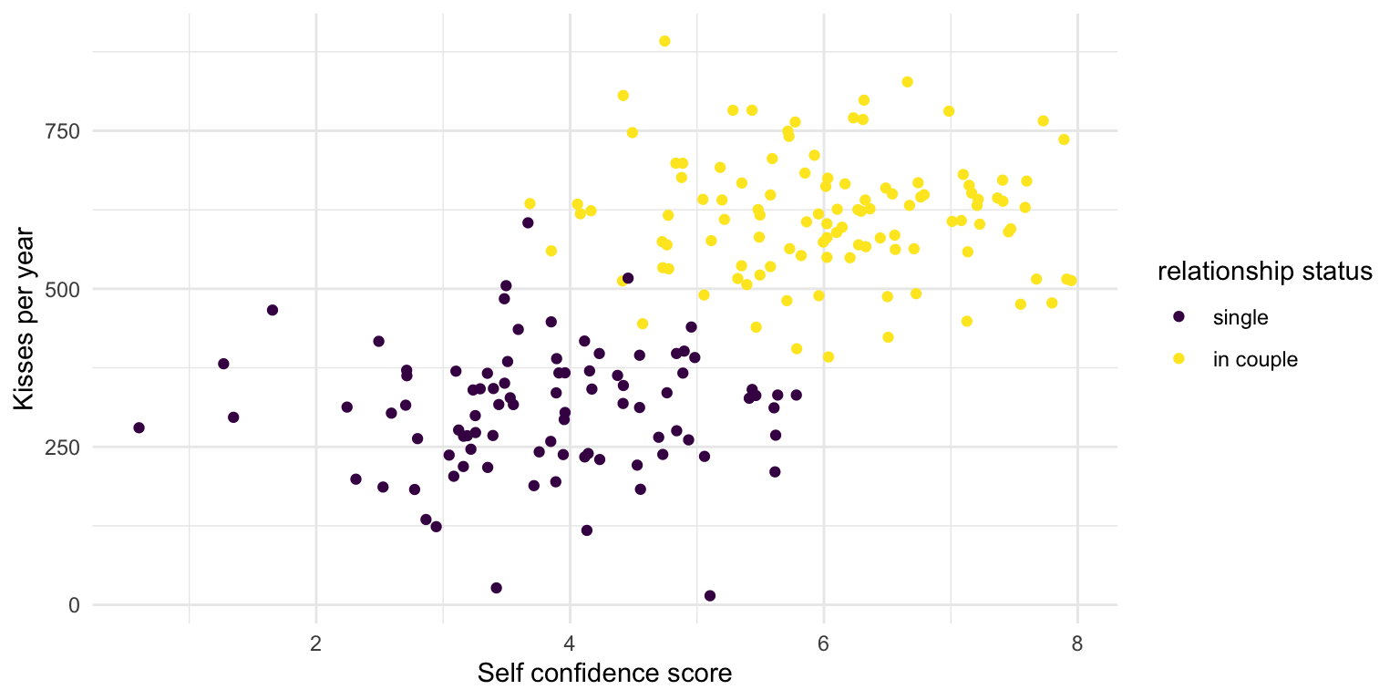
No more relationship within the different subgroups
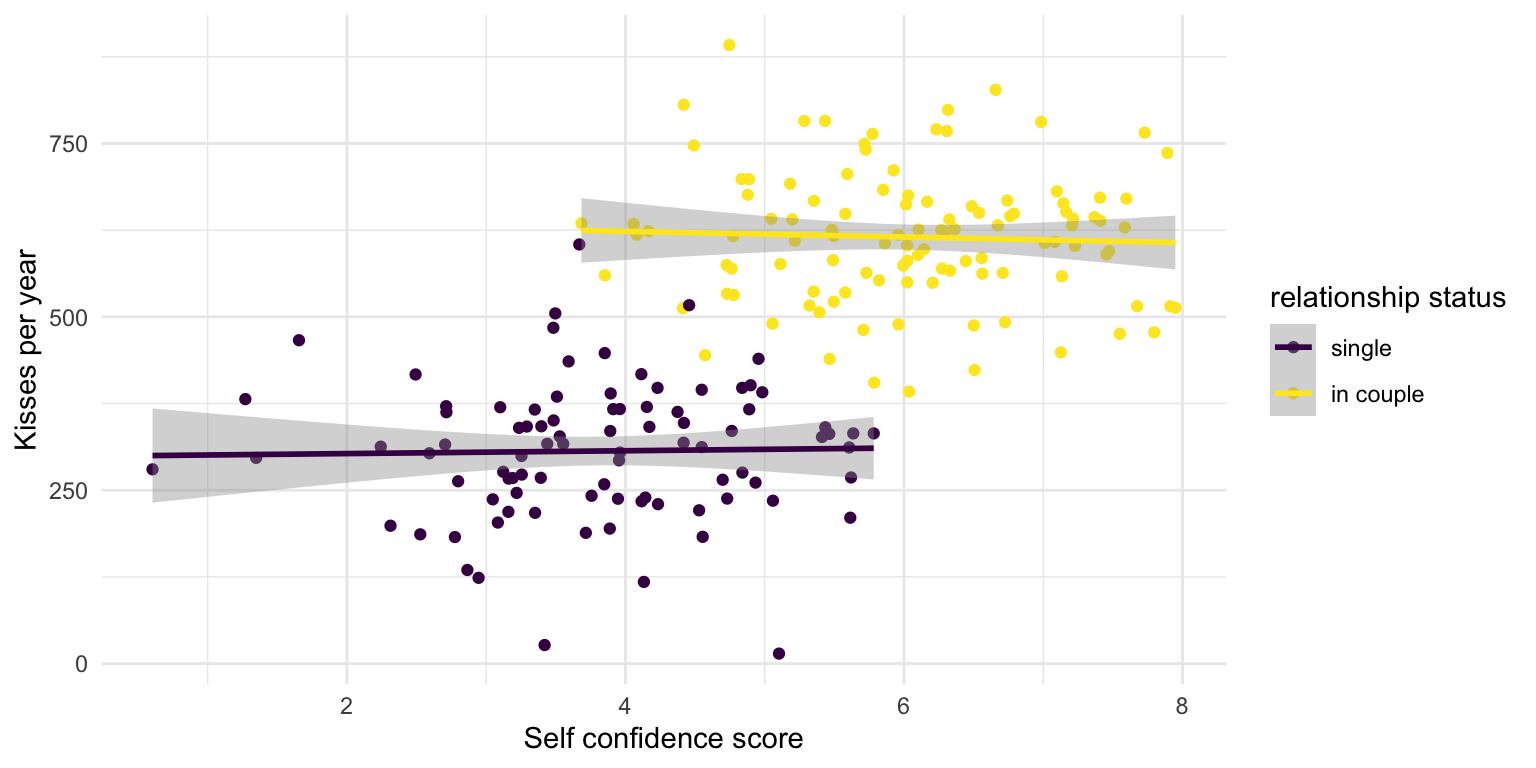
In fact, this is how the data was generated
Relationship status increases both kisses and self confidence. They are otherwise independent.
set.seed(1234) # For reproducibility

sample_size <- 200

kisses <- tibble(
  id = 1:sample_size,
  relationship = sample(0:1, sample_size, replace = TRUE),
  # we use rtruncnorm() to add some random variation
  # a and b arguments in rtruncnorm() mark the limits of the sampling
  kisses = 300 + 300*relationship + rtruncnorm(sample_size, mean = 0, sd = 100, a = - 300),
  self_confidence = 4 + 2*relationship + rtruncnorm(sample_size, mean = 0, sd = 1, a = - 4, b = 2)
) |>
  # pick nicer values for the relationship variable
  mutate(relationship = recode_factor(relationship, `0` = "single",
                                      `1` = "in couple"))
Relationship status is a “Confounder”
To account for confounders, in a regression analysis, we can add it as another predictor to our regression model.
People also call this “controlling for a variable”
This is like looking into the two groups (relationship vs. single) separately.
Relationship status is a “Confounder”
Call:
lm(formula = kisses ~ self_confidence + relationship, data = kisses)

Residuals:
     Min       1Q   Median       3Q      Max
-290.439  -63.130    6.422   57.785  297.704

Coefficients:
                      Estimate Std. Error t value Pr(>|t|)
(Intercept)            311.300     27.773  11.209   <2e-16 ***
self_confidence         -1.261      6.786  -0.186    0.853
relationshipin couple  311.225     20.566  15.133   <2e-16 ***
---
Signif. codes:  0 '***' 0.001 '**' 0.01 '*' 0.05 '.' 0.1 ' ' 1

Residual standard error: 97.25 on 197 degrees of freedom
Multiple R-squared:  0.7165,    Adjusted R-squared:  0.7136
F-statistic: 248.9 on 2 and 197 DF, p-value: < 2.2e-16- Our research question was about a causal effect of self confidence, so we only interpret the
self_confidenceestimate. Note how the effect is tiny now, and statistically not significantly different from 0.
Note
As a rule, never interpret the estimates of control variables in regressions. Focus on the one variable that your research question was on.
Confounders
In sum we want to control for confounders in our analyses
Colliders
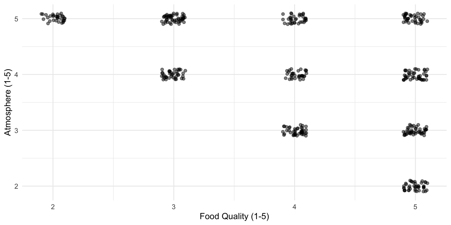
Are shabby-looking restaurants serving nicer food than fancy ones?
Imagine that’s your research question.
You know that restaurants in your town are rated based on two criteria: food quality and atmosphere.
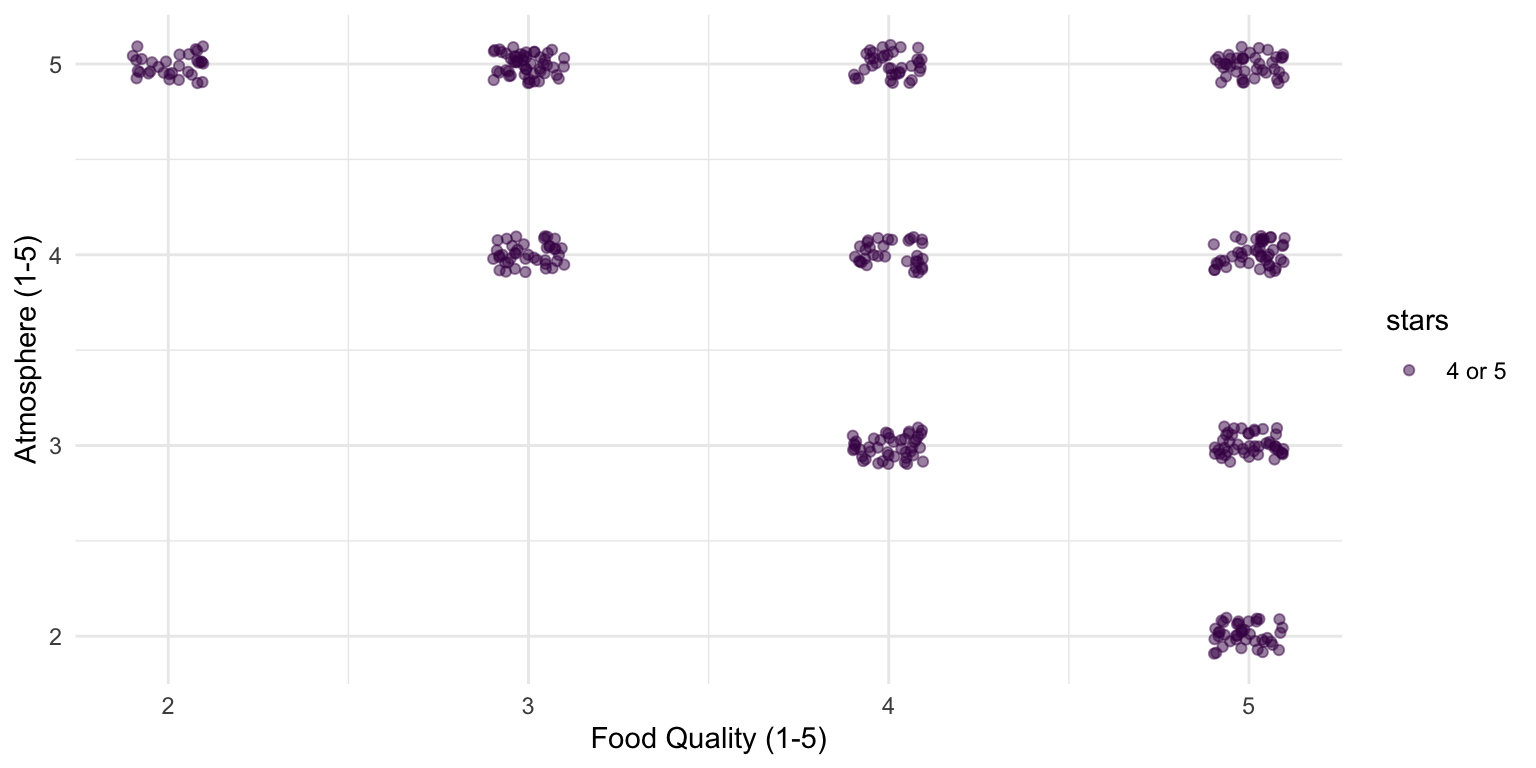
You check out all the greatest restaurants in town (at least 4 out of 5 stars) and this is what you observe:
Data of 4- and 5-star restaurants
There appears to be a relationship!
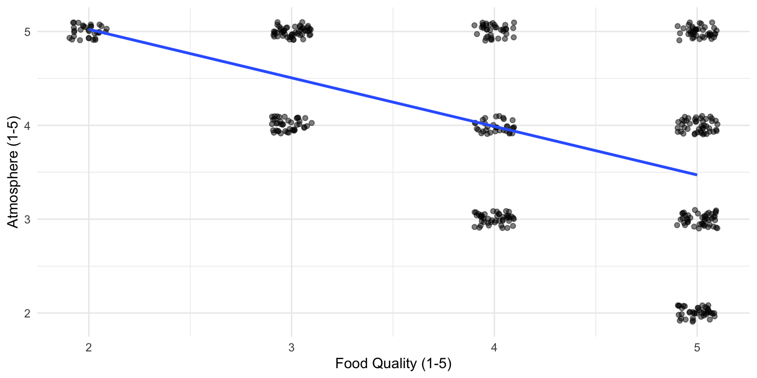
But remember, we are only looking at the best restaurants
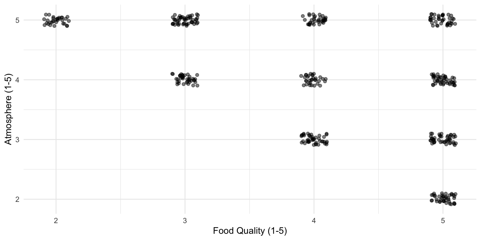
Yet, our research questions was about restaurants in general
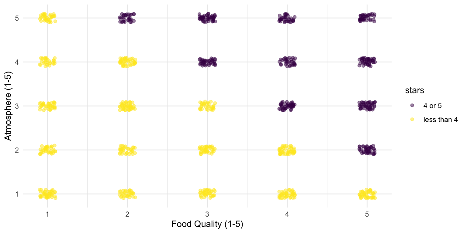
When looking at all restaurants, there is no relationship
In fact, this is how the data was generated
sample_size <- 1000
# Generate independent food quality and atmosphere scores (1 to 5)
restaurants <- tibble(
id = 1:sample_size,
food_quality = sample(1:5, sample_size, replace = TRUE),
atmosphere = sample(1:5, sample_size, replace = TRUE),
# Overall rating depends on both factors (rounded to nearest integer)
rating = round((food_quality + atmosphere) / 2 )
) |>
# add an additional variable of whether 4 or more stars
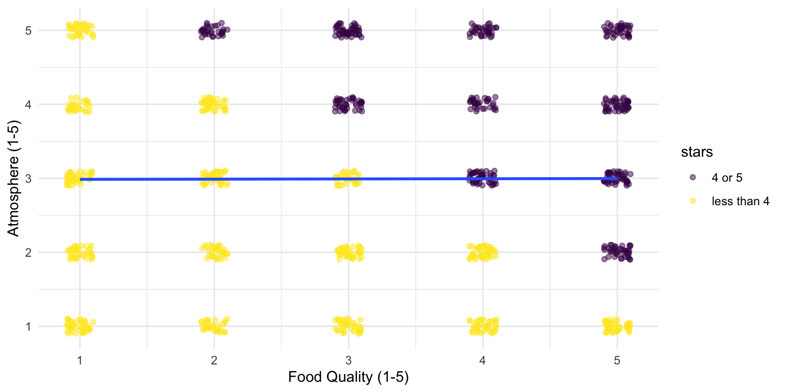
mutate(stars = ifelse(rating >= 4, "4 or 5", "less than 4"))Restaurant stars is a “Collider variable”
If we look at only the best restaurants, our model yields a statistically significant negative association.
best_restaurants <- restaurants |>
  filter(stars == "4 or 5")

model <- lm(atmosphere ~ food_quality, data = best_restaurants)

tidy(model)
# A tibble: 2 × 5
term estimate std.error statistic p.value
<chr> <dbl> <dbl> <dbl> <dbl>
1 (Intercept) 6.06 0.183 33.2 2.16e-118
2 food_quality -0.517 0.0439 -11.8 8.30e- 28Note that this similar to adding stars as a control variable (for both subgroups, selecting them independently yields a negative relationship)
# A tibble: 3 × 5
  term             estimate std.error statistic   p.value
  <chr>               <dbl>     <dbl>     <dbl>     <dbl>
1 (Intercept)         5.94     0.120       49.4 2.71e-270
2 food_quality       -0.488    0.0271     -18.0 7.81e- 63
3 starsless than 4   -2.47     0.0781     -31.6 1.91e-152
Restaurant stars is a “Collider variable”
If we look at all restaurants, our model will yield no statistically significant association (in line with the true data generating process).
Colliders
We do not want to control/condition on colliders in our analyses.
Note
Note that the restaurant case we have discussed is a special case of collider bias, which is called a selection bias. The idea behind a name is that you select a non-random sample of a population that you want to make claims about.
That’s it for today :)