

05:00
Meta Analyses
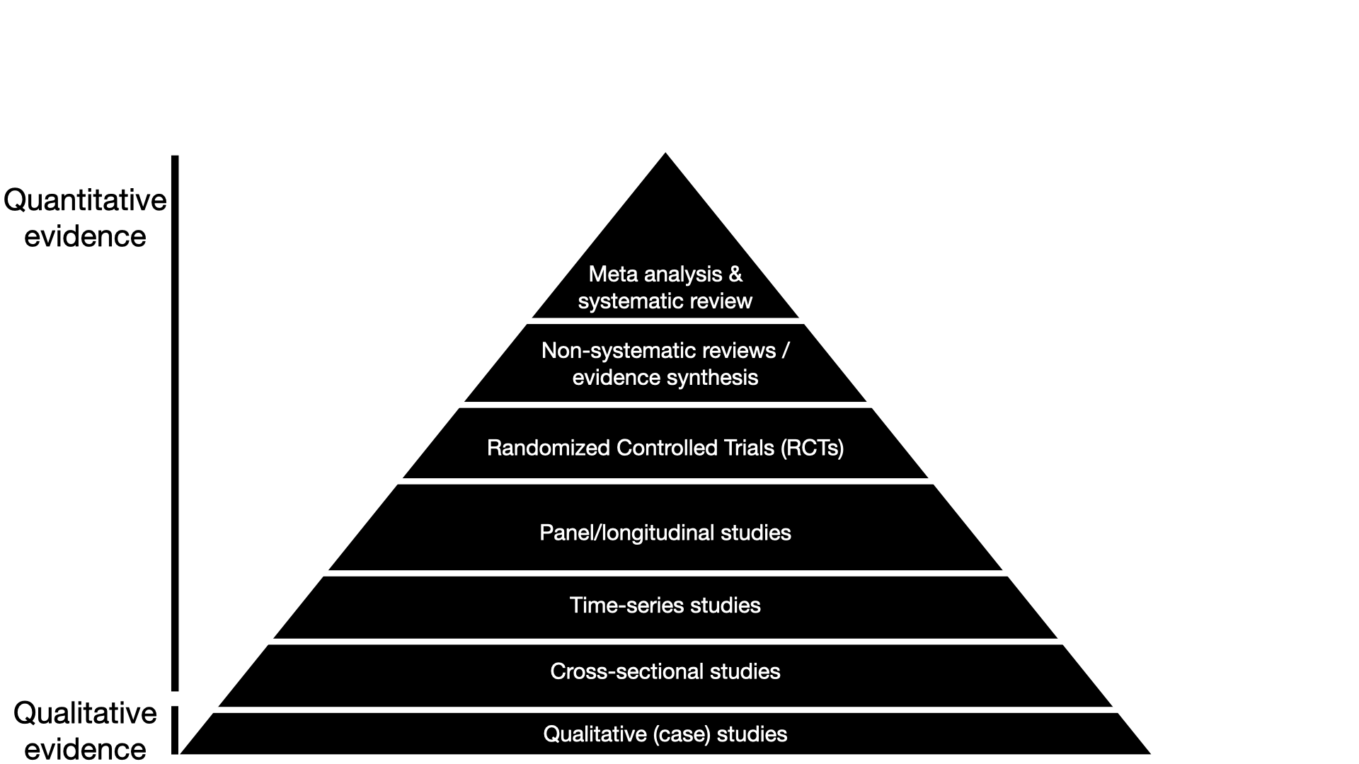
(A typical textbook) pyramid of evidence
Case study: “Can people tell true news from false News ?”
What are effect sizes?
In Meta-analyses not individual participants, but single studies are the unit of analysis
The outcomes of these studies are called “effect sizes”.
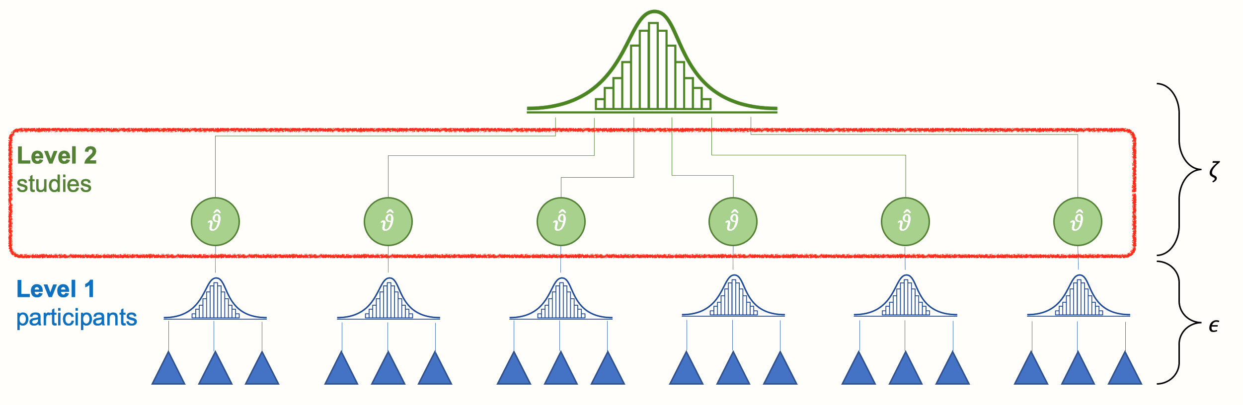
Graphic adapted from: Harrer, M., Cuijpers, P., A, F. T., & Ebert, D. D. (2021). Doing Meta-Analysis With R: A Hands-On Guide (1st ed.). Chapman & Hall/CRC Press.
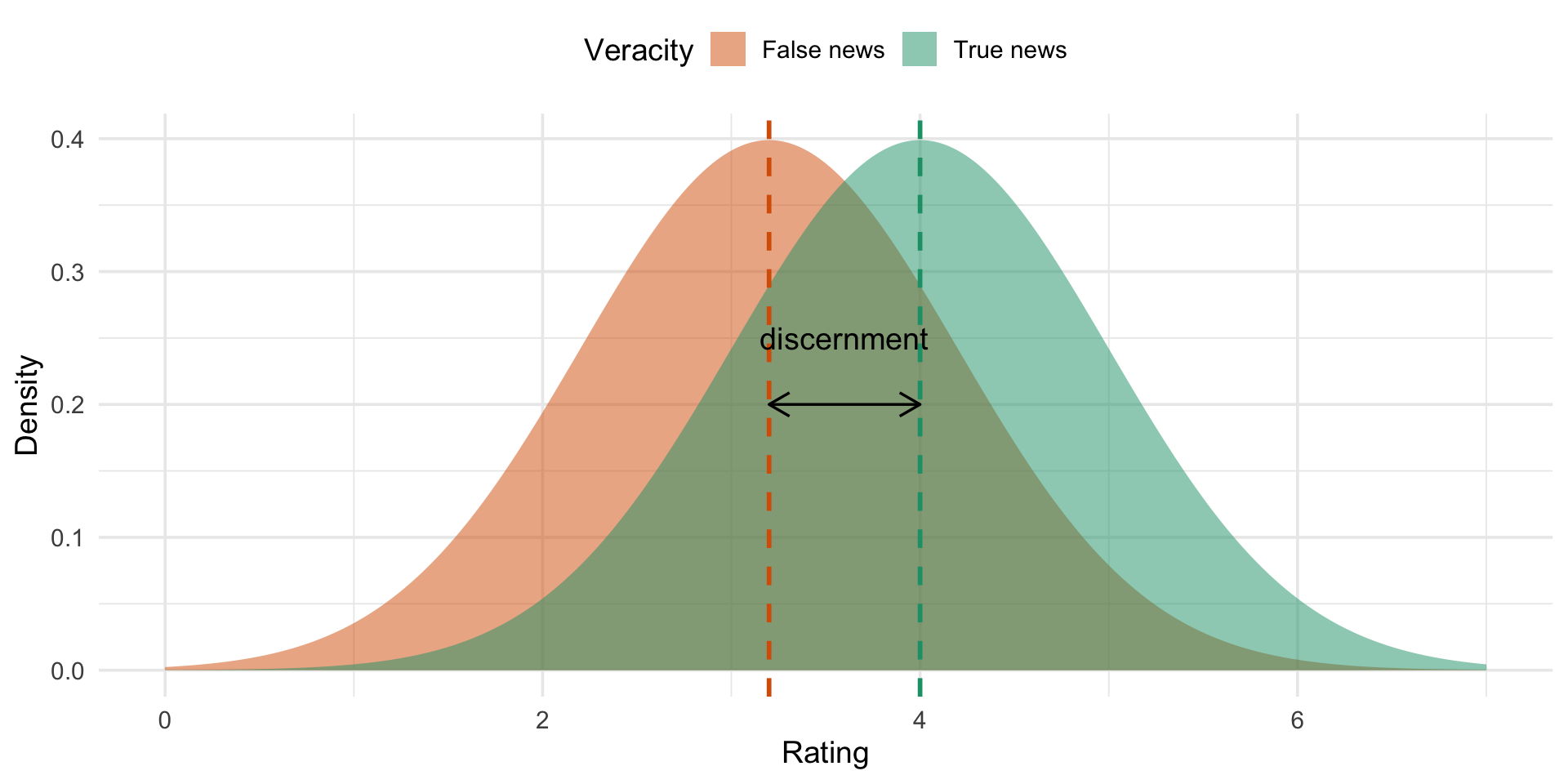
Cohen’s d
If we plot the distribution of all individual accuracy ratings, we get something like below (slightly less perfect).
Cohen’s d uses the standard devations of these distributions
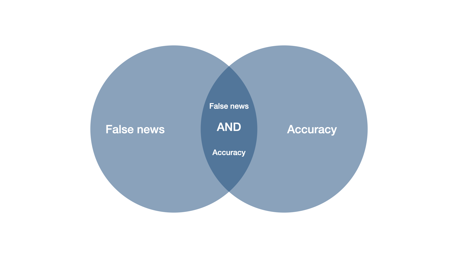
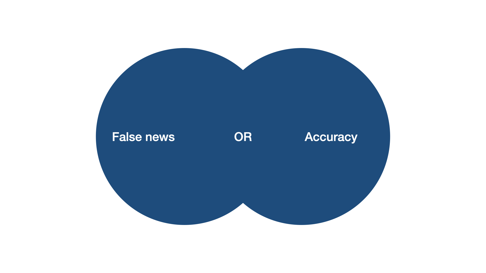
The search string
Ideally, we want all studies that have ever been written on our research question. The more the better.
But…

We often need to be specific in our search.
Boolean operators
Data bases
Data bases allow very refined searches.
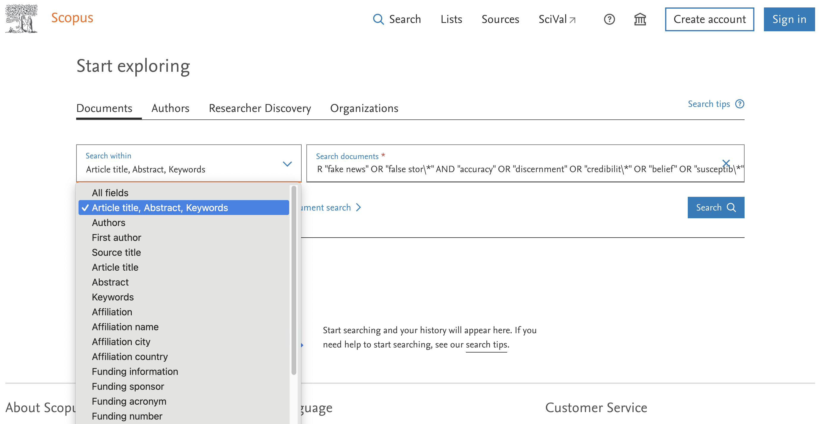
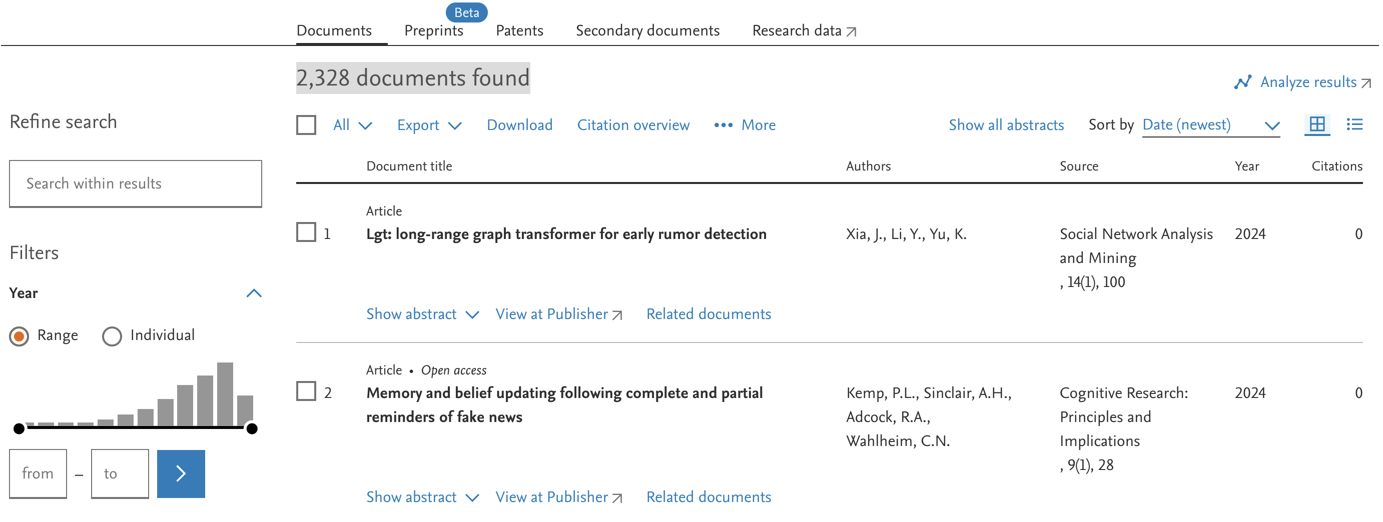
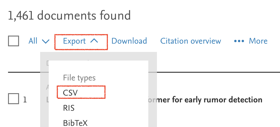
Data bases
Some databases also have features to export your search results as data sets.
The meta-analytic average
- A meta-analysis is basically taking an average of all effect sizes
Graphic adapted from: Harrer, M., Cuijpers, P., A, F. T., & Ebert, D. D. (2021). Doing Meta-Analysis With R: A Hands-On Guide (1st ed.). Chapman & Hall/CRC Press.
Forest plot
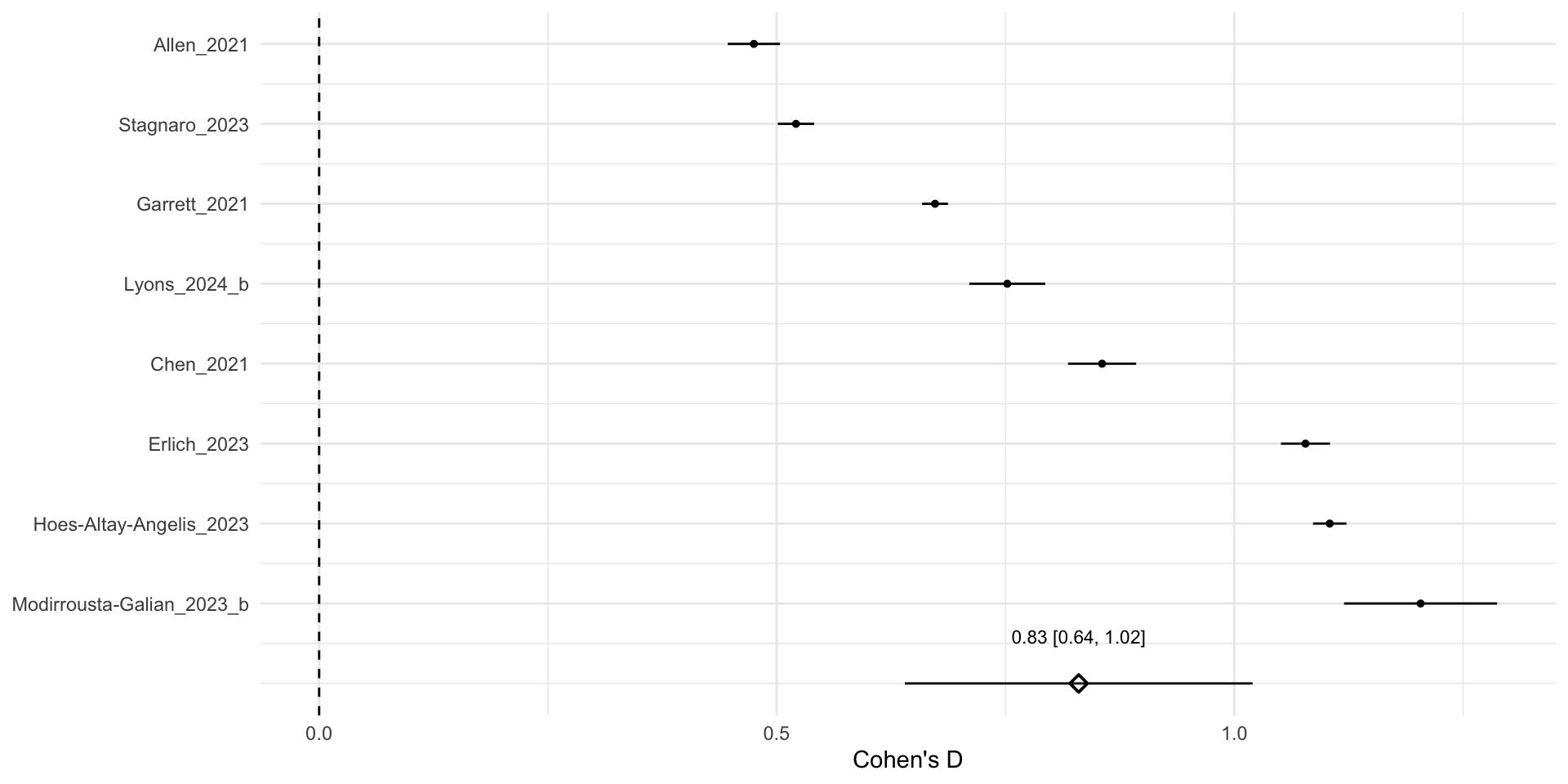
Points are effect sizes, bars are 95% confidence intervals - an indicator of statistical significance we haven’t discussed yet. The idea is that if they exclude 0, that’s like having a p-value below 0.05: the estimate is statistically significant.