Statistical Power

Overview

1. The Central Limit Theorem revisited

2. From Null worlds to True effect worlds

3. Statistical power

4. A power simulation

The Central Limit Theorem revisited

Are action movies better than comedies?

In the previous session on hypothesis testing, we invented a null world:

We simulated a population of 1’000’000 movies with no difference.

set.seed(1234) # For reproducibility

imaginary_movies_null <- tibble(
  movie_id = 1:1000000,
  rating = sample(seq(1, 10, by = 0.1), size = 1000000, replace = TRUE),
  genre = sample(c("Comedy", "Action"), size = 1000000, replace = TRUE)
)

Sampling distribution

We randomly drew 1,000 samples from this population and calculated the difference between action movies and comedies for each.

We called the distribution of the differences from the different samples the sampling distribution

Our sample size was always the same: 20,000.

n_simulations <- 1000
differences <- c() # make an empty vector
sample_size <- 20000

for (i in 1:n_simulations) {
  # draw a sample of 20'000 films
  imaginary_sample <- imaginary_movies |> 
    sample_n(sample_size)
  # compute rating difference in the sample
  estimate <- imaginary_sample |> 
    group_by(genre) |> 
    summarize(avg_rating = mean(rating)) |> 
    summarise(diff = avg_rating[genre == "Action"] - avg_rating[genre == "Comedy"]) %>%
    pull(diff)
  
  differences[i] <- estimate
}

The Central Limit Theorem (part I)

The sampling distribution approximates the shape of a normal distribution

The Central Limit Theorem (part II)

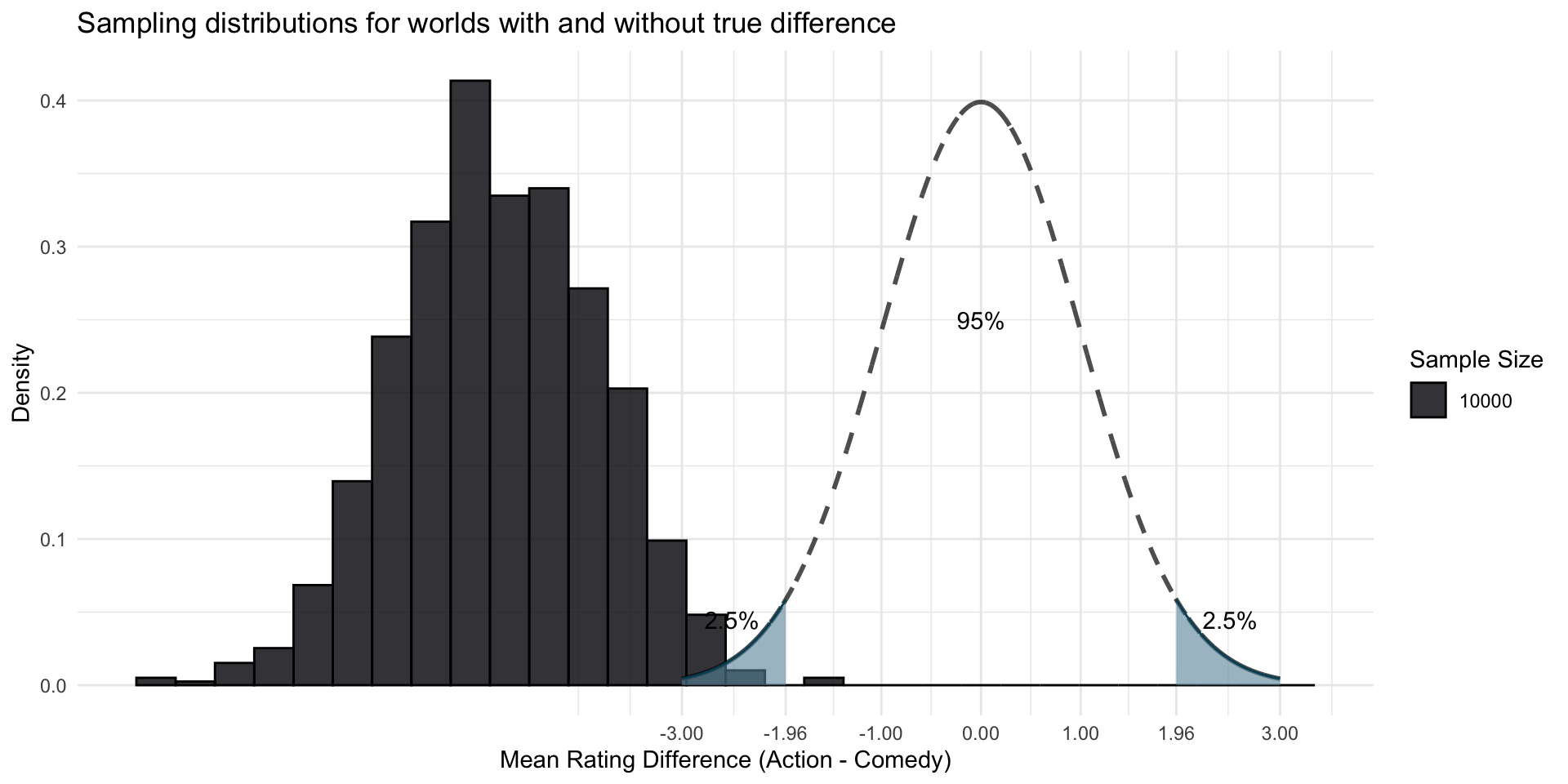
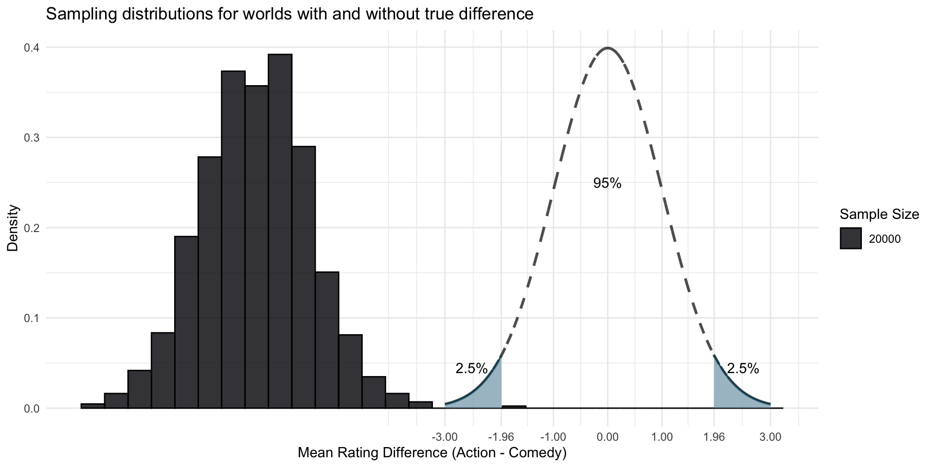
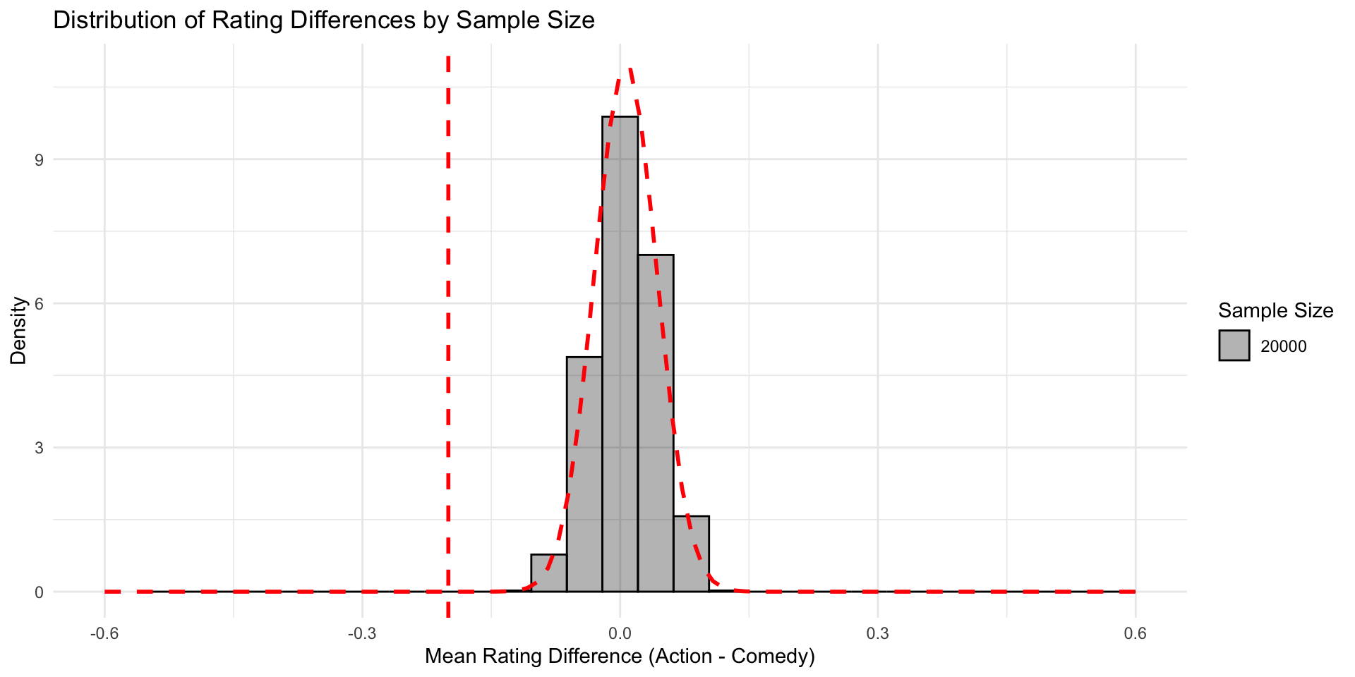
This is what the sampling distribution looks like with samples of size 10,000

The Central Limit Theorem (part II)

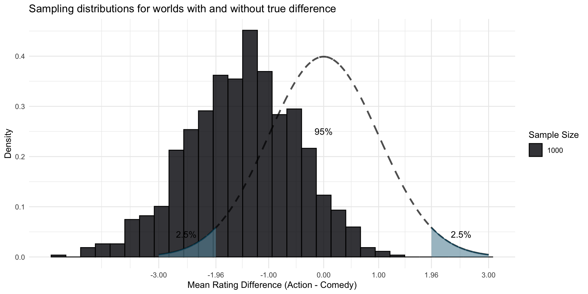
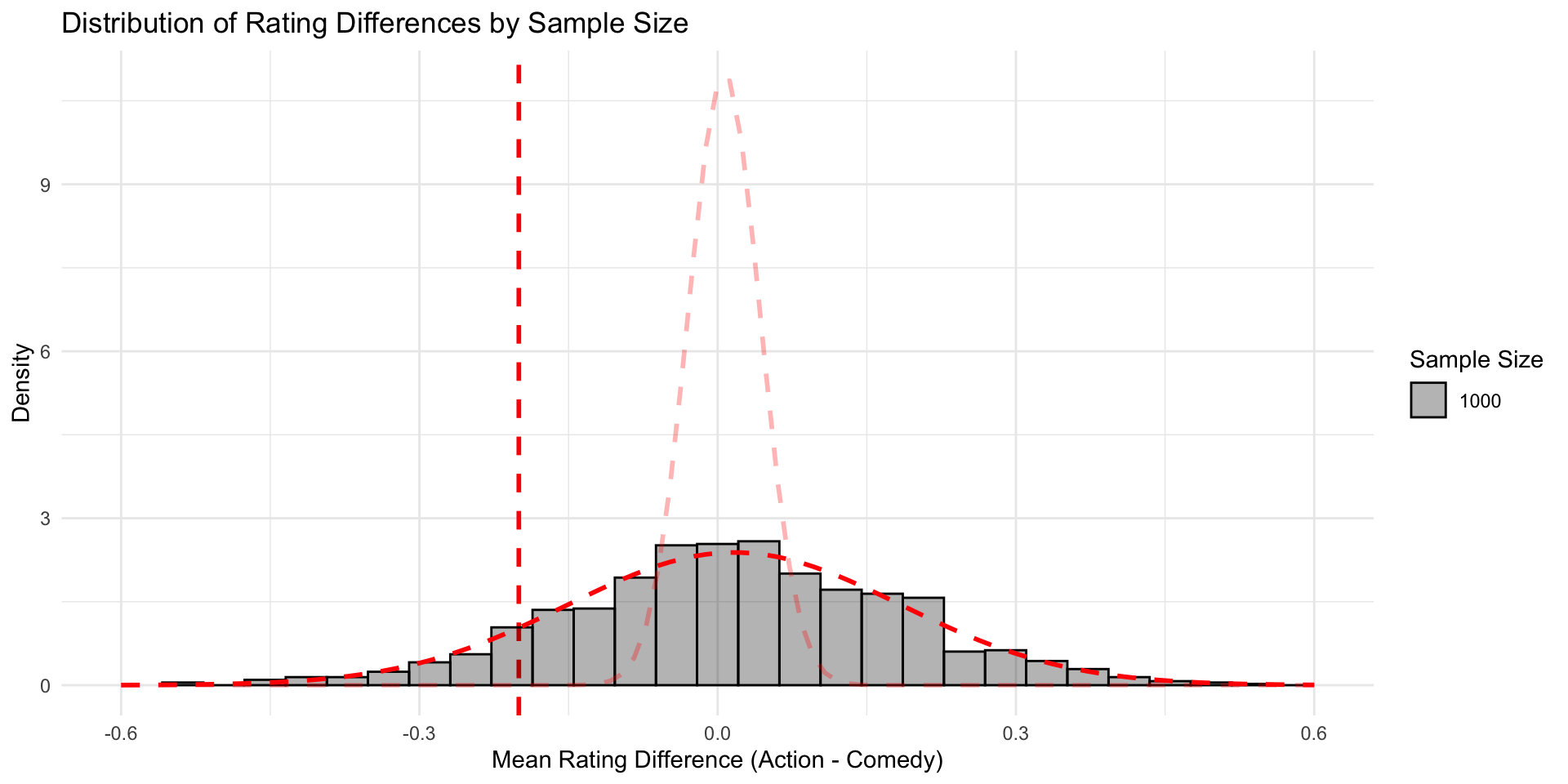
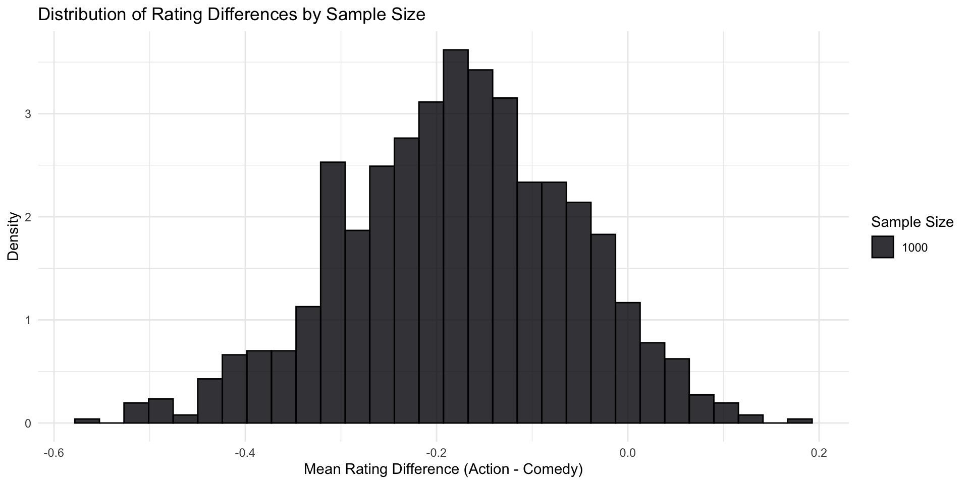
And with samples of size 1,000

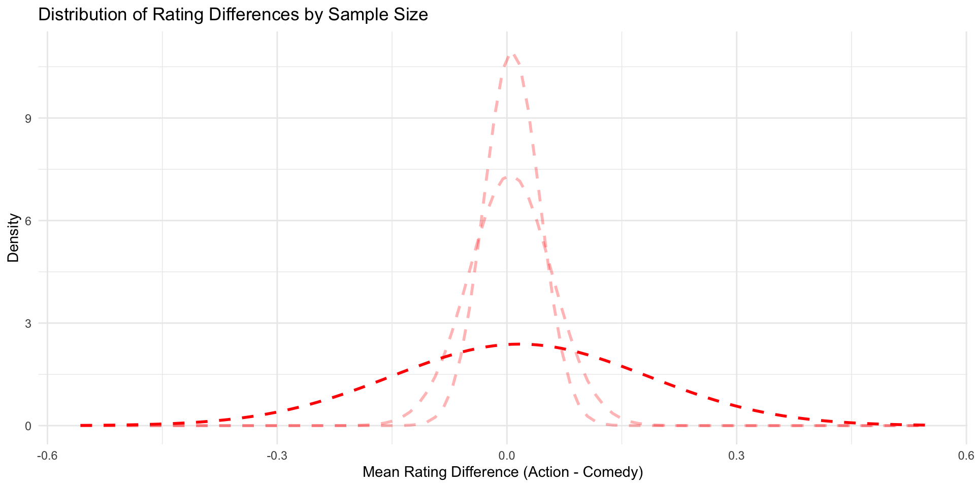
The Central Limit Theorem (part II)

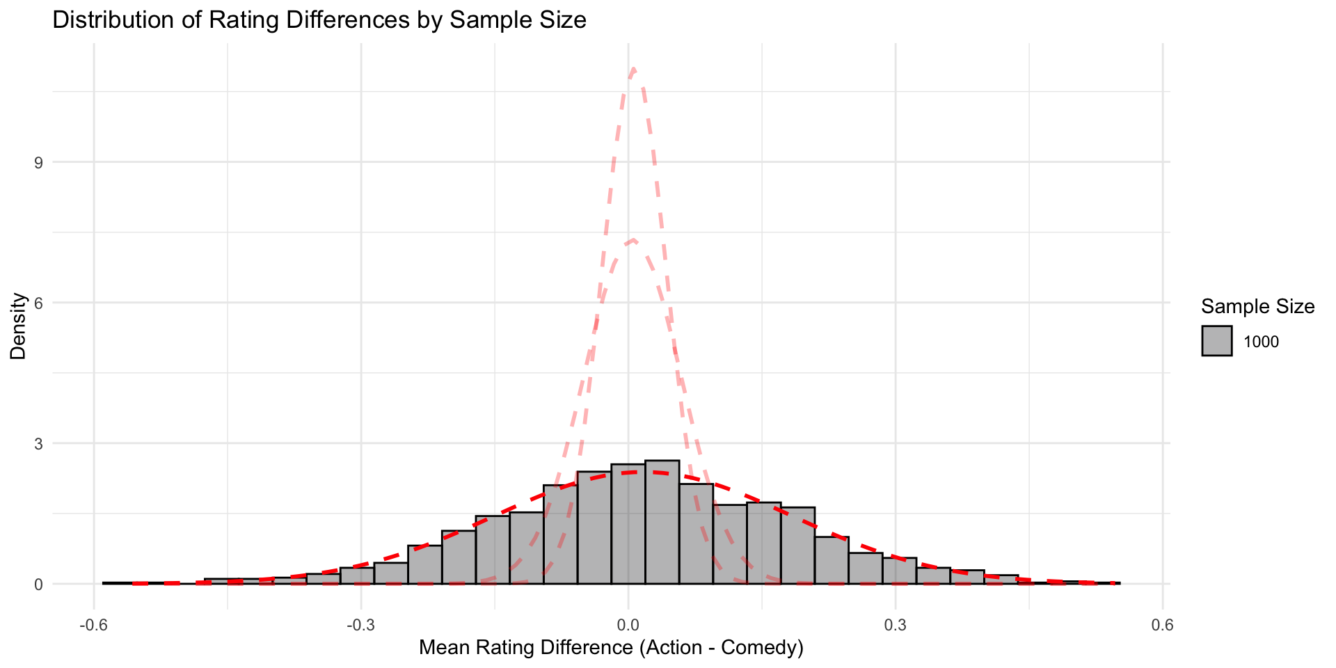
The smaller the sample, the larger the standard deviation of the sampling distribution

How is this relevant for hypothesis testing?

Imagine we find an effect of -0.2 in our sample

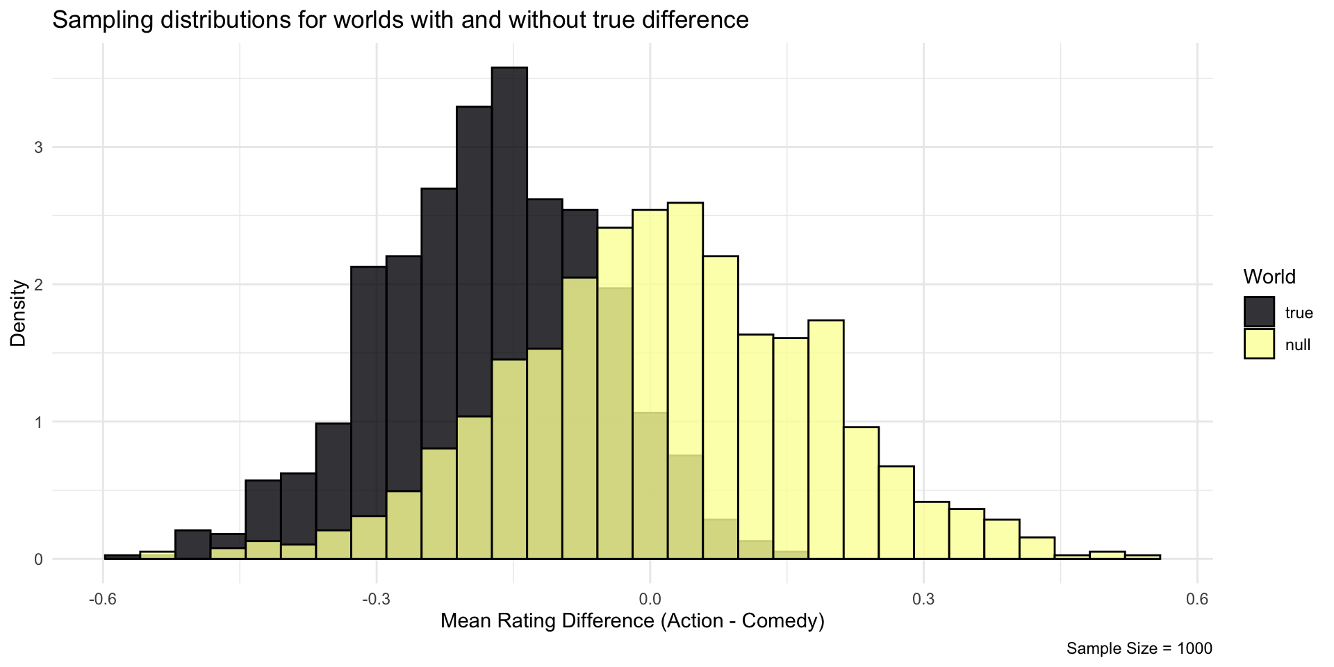
In a sample based on 20’000 movies, that seems reasonably unlikely in a Null world

But the same effect in a sample of 1000 seems not so unlikely…

The Central Limit Theorem

(part I)

• The sampling distribution approximates the shape of a normal distribution

(part II)

• The smaller the sample, the larger the standard deviation of the sampling distribution

From Null worlds to True effect worlds

For example, let’s imagine a world where the true difference between action and comedy movies is -0.2

# Generate Comedy and Action movie ratings using truncated normal distributions
imaginary_movies_true <- tibble(
  movie_id = 1:1000000,
  genre = sample(c("Comedy", "Action"), size = 1000000, replace = TRUE),
  rating = ifelse(
    genre == "Comedy",
    rtruncnorm(1000000, a = 1, b = 10, mean = 6.0, sd = 2), 
    rtruncnorm(1000000, a = 1, b = 10, mean = 5.8, sd = 2)   
  )
)

Let’s plot the population data

# Compute means
means <- imaginary_movies_true |> 
  group_by(genre) |> 
  summarize(mean_rating = mean(rating)) |> 
  # Adjust vertical placement for text labels
  mutate(label_y = c(0.08, 0.06)) 

# Plot
ggplot(imaginary_movies_true, aes(x = rating, fill = genre)) +
  geom_histogram(aes(y = ..density..), bins = 30, alpha = 0.5, position = "identity") +
  scale_fill_viridis_d(option = "plasma", begin = 0.2, end = 0.8) +  # Viridis color scale
  scale_color_viridis_d(option = "plasma", begin = 0.2, end = 0.8) +  # Viridis color scale
  geom_vline(data = means, aes(xintercept = mean_rating, color = genre), 
             linetype = "dashed", size = 1, show.legend = FALSE) +  # Remove color legend for lines 
  geom_text(data = means, aes(x = mean_rating, y = label_y, label = round(mean_rating, 2)),
            hjust = -0.1, fontface = "bold") +  # Adjusted position to avoid overlap
  labs(title = "Distribution of Movie Ratings by Genre",
       x = "Rating",
       y = "Density",
       fill = "Genre") +
  theme_minimal()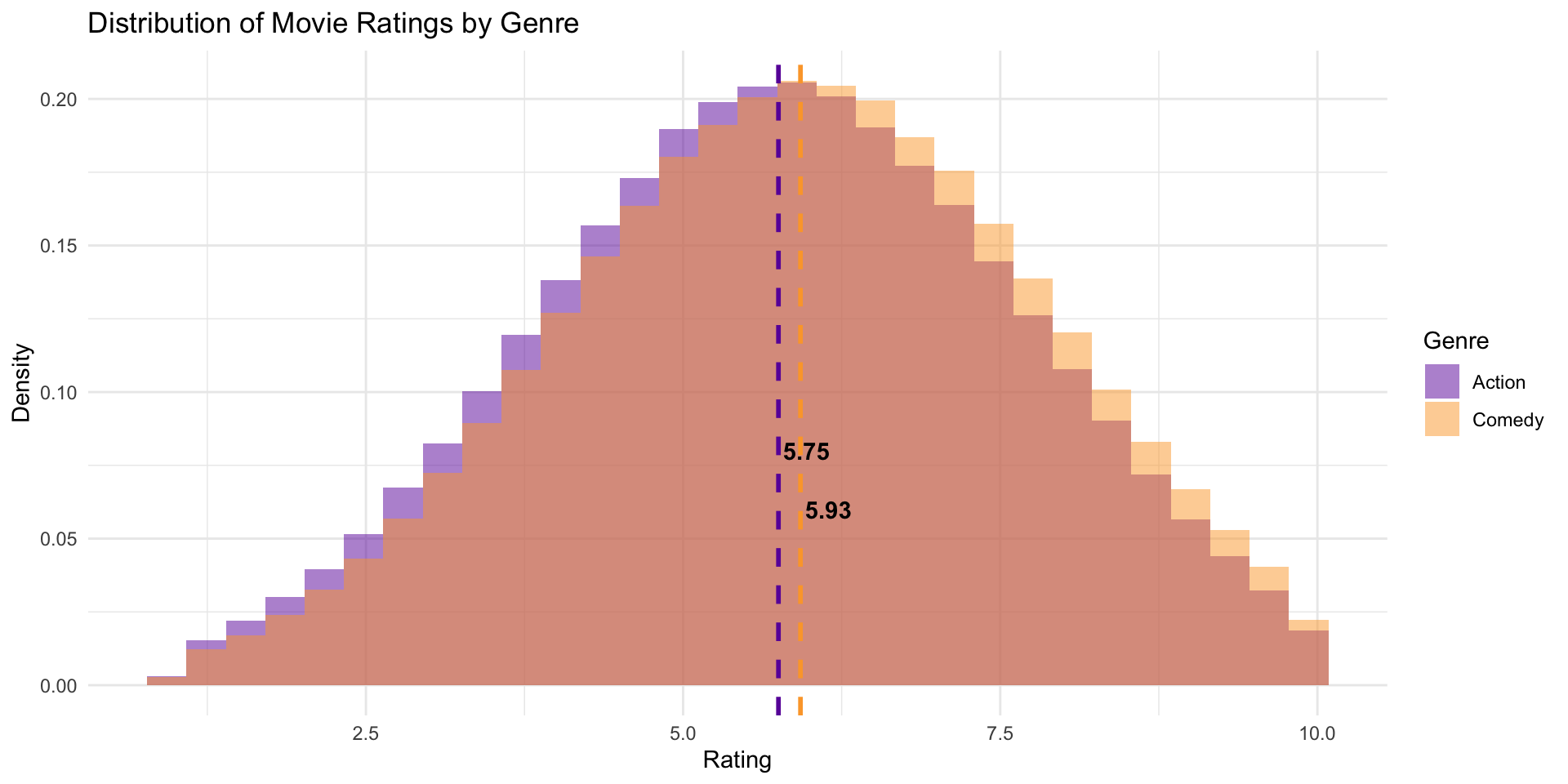 

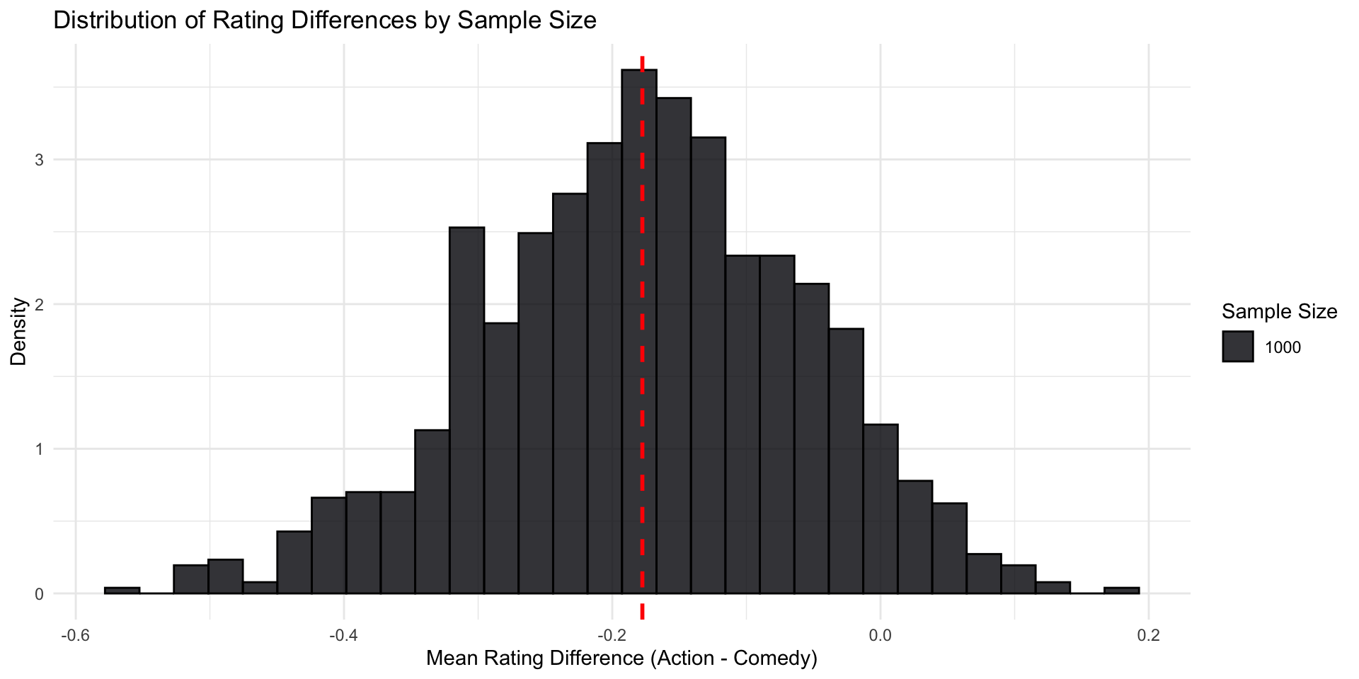
🎉 It worked, we see our imagined effect of ~ -0.2

# Compute means
means <- imaginary_movies_true |> 
  group_by(genre) |> 
  summarize(mean_rating = mean(rating)) |> 
  # Adjust vertical placement for text labels
  mutate(label_y = c(0.08, 0.06)) 

# Plot
ggplot(imaginary_movies_true, aes(x = rating, fill = genre)) +
  geom_histogram(aes(y = ..density..), bins = 30, alpha = 0.5, position = "identity") +
  scale_fill_viridis_d(option = "plasma", begin = 0.2, end = 0.8) +  # Viridis color scale
  scale_color_viridis_d(option = "plasma", begin = 0.2, end = 0.8) +  # Viridis color scale
  geom_vline(data = means, aes(xintercept = mean_rating, color = genre), 
             linetype = "dashed", size = 1, show.legend = FALSE) +  # Remove color legend for lines 
  geom_text(data = means, aes(x = mean_rating, y = label_y, label = round(mean_rating, 2)),
            hjust = -0.1, fontface = "bold") +  # Adjusted position to avoid overlap
  labs(title = "Distribution of Movie Ratings by Genre",
       x = "Rating",
       y = "Density",
       fill = "Genre") +
  theme_minimal() 

Imagine we look at a sample of 1000 movie ratings.

n_simulations <- 1000
differences <- c() # make an empty vector
sample_size <- 1000

for (i in 1:n_simulations) {
  # draw a sample of 20'000 films
  imaginary_sample <- imaginary_movies |> 
    sample_n(sample_size)
  # compute rating difference in the sample
  estimate <- imaginary_sample |> 
    group_by(genre) |> 
    summarize(avg_rating = mean(rating)) |> 
    summarise(diff = avg_rating[genre == "Action"] - avg_rating[genre == "Comedy"]) %>%
    pull(diff)
  
  differences[i] <- estimate
}

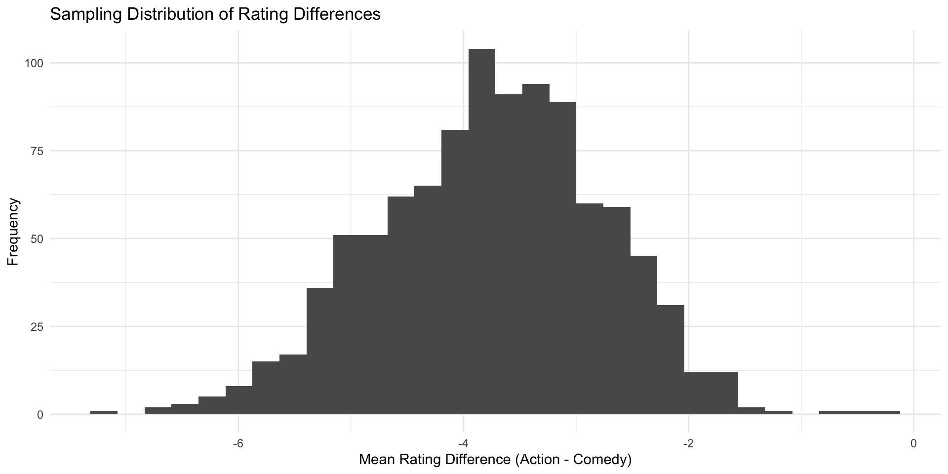
This is what our sampling distribution would look like

Now imagine we do a hypothesis test.

We can simulate both a null world and a true effect world (so far, nothing new)

Null world

# Null world population
imaginary_movies_null <- tibble(
  movie_id = 1:1000000,
  rating = sample(seq(1, 10, by = 0.1), size = 1000000, replace = TRUE),
  genre = sample(c("Comedy", "Action"), size = 1000000, replace = TRUE)
)

True effect world

# True effect world population
imaginary_movies_true <- tibble(
  movie_id = 1:1000000,
  genre = sample(c("Comedy", "Action"), size = 1000000, replace = TRUE),
  rating = ifelse(
    genre == "Comedy",
    rtruncnorm(1000000, a = 1, b = 10, mean = 6.0, sd = 2), 
    rtruncnorm(1000000, a = 1, b = 10, mean = 5.8, sd = 2)   
  )
)

And make a sampling distribution with sample size 1000 for both worlds (also nothing new)

n_simulations <- 1000
differences <- c() # make an empty vector
sample_size <- 1000

data <- imaginary_movies_true # replace with imaginary_movies_null

for (i in 1:n_simulations) {
  # draw a sample of films
  imaginary_sample <- data |> 
    sample_n(sample_size)
  # compute rating difference in the sample
  estimate <- imaginary_sample |> 
    group_by(genre) |> 
    summarize(avg_rating = mean(rating)) |> 
    summarise(diff = avg_rating[genre == "Action"] - avg_rating[genre == "Comedy"]) %>%
    pull(diff)
  
  differences[i] <- estimate
}

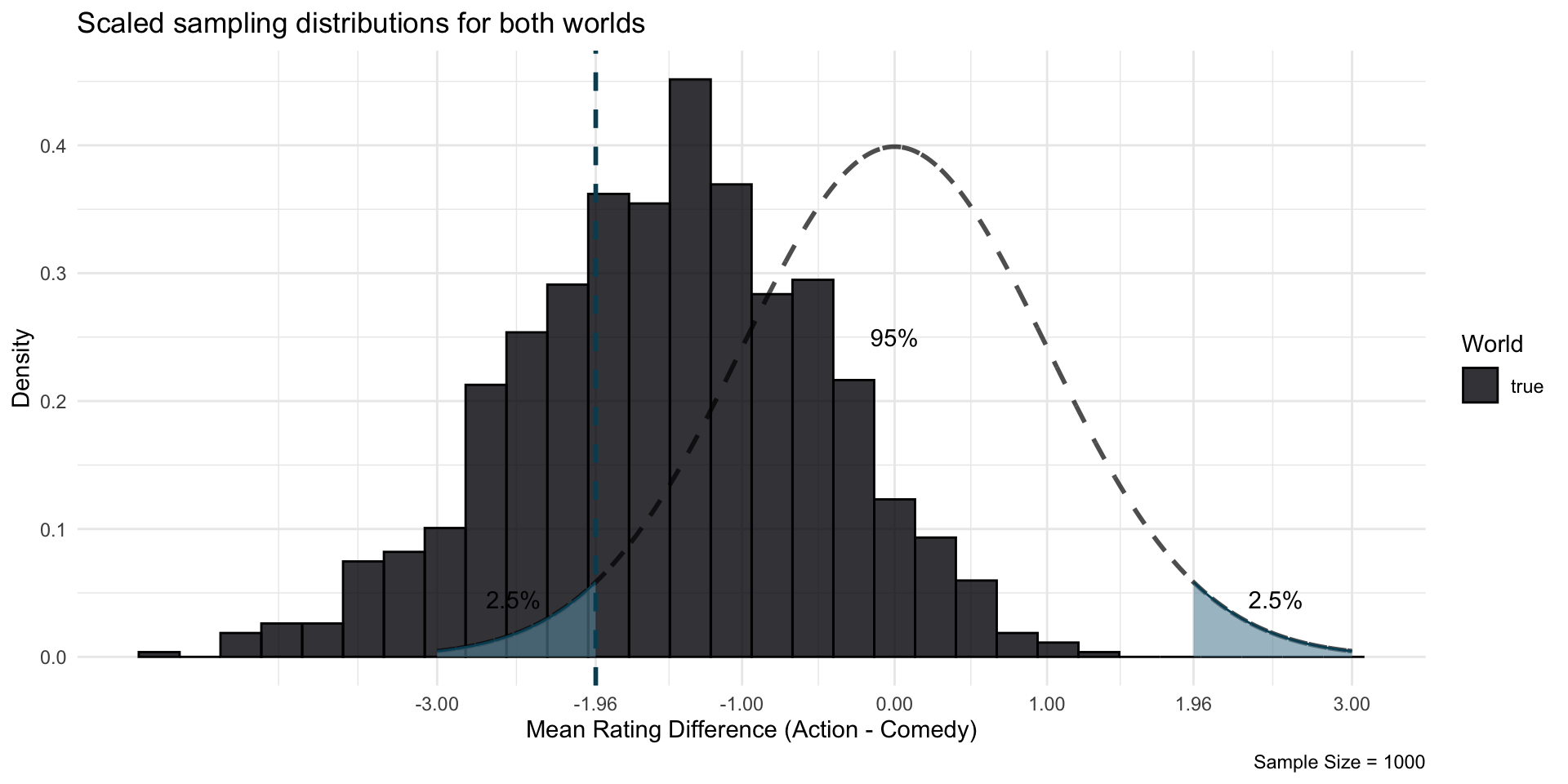
We can plot both simulated worlds together.

Let’s bring both worlds on the scale of a standard normal distribution, dividing their respective standard deviation

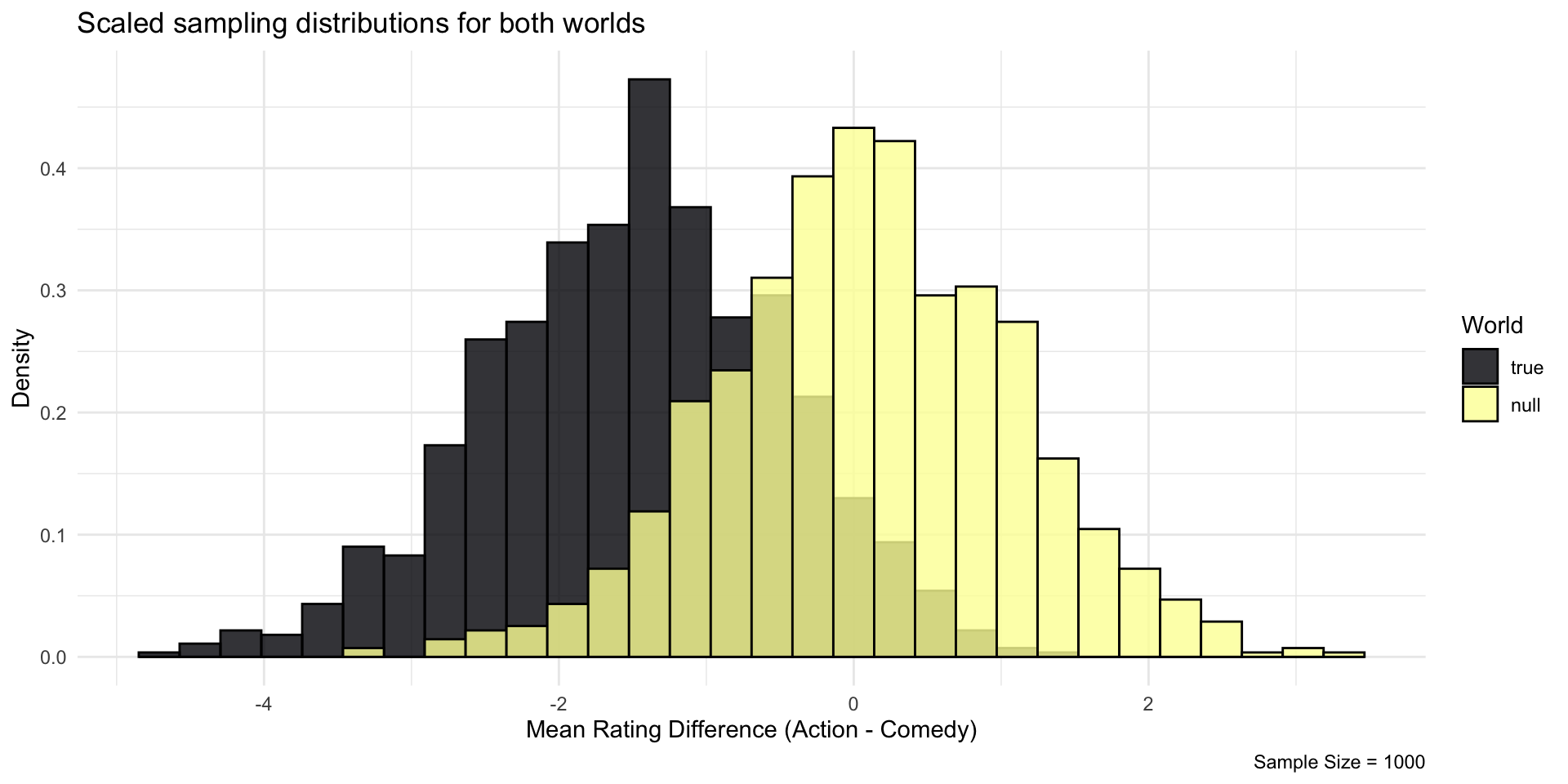
With a sample size of 1000, in many cases, we would say: “This could have occurred in a Null World”

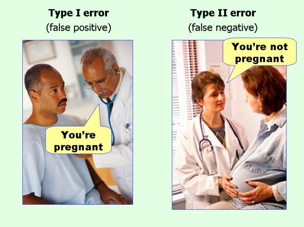
Two errors

Hypothesis Testing

Statistical Power

Two errors

	Hypothesis Testing	Power Analysis
Aim	Rule out that we observe something just by chance.	Ensure that we would find an effect.
Error question	“What are the chances that we find an effect at least this large in our sample, given that there is no effect in the population?”	“What are the chances that we do not find a statistically significant effect in our sample, although there is a certain effect in the population?”
Typical threshold for acceptable error	\(\alpha\) = 5 %	\(\beta\) = 20 %

Statistical Power

Statistical Power

Statistical power is the probability of detecting an effect with a hypothesis test, given a certain effect size

(Or \(1 - \beta\))

Your turn #1: Calculating power

1. Create your true effect world: Simulate a population with a true difference of -0.5 between action and comedy movies.

2. Get your sampling distribution: Simulate 1000 random samples of size n = 1000 and store the results.

3. Plot your Sampling distribution (use data.frame() to turn your vector into a data frame that can be read by ggplot)

4. Prepare for hypothesis testing: bring the results on scale of the standard normal distribution (divide by the standard deviation of your distribution)

5. Check the transformation: plot the new, standardized values

6. Calculate your power: Check how many (standardized) differences are below the 5% threshold, i.e. smaller than or equal to -1.96 (hint: use mutate() in combination with ifelse to create a new variable significant that takes the values of TRUE or FALSE. Then use summarize() and sum() to calculate the share). Are you above the 80% power threshold?

15:00

1. Create your true effect world: Simulate a population with a true difference of -0.5 between action and comedy movies.

# True effect world population
imaginary_movies_true <- tibble(
  movie_id = 1:1000000,
  genre = sample(c("Comedy", "Action"), size = 1000000, replace = TRUE),
  rating = ifelse(
    genre == "Comedy",
    rtruncnorm(1000000, a = 1, b = 10, mean = 6.0, sd = 2), 
    rtruncnorm(1000000, a = 1, b = 10, mean = 5.5, sd = 2)   
  )
)

2. Get your sampling distribution: Simulate 1000 random samples of size n = 1000 and store the results.

n_simulations <- 1000
differences <- c() # make an empty vector
sample_size <- 1000

data <- imaginary_movies_true # replace with imaginary_movies_null

for (i in 1:n_simulations) {
  # draw a sample of films
  imaginary_sample <- data |> 
    sample_n(sample_size)
  # compute rating difference in the sample
  estimate <- imaginary_sample |> 
    group_by(genre) |> 
    summarize(avg_rating = mean(rating)) |> 
    summarise(diff = avg_rating[genre == "Action"] - avg_rating[genre == "Comedy"]) %>%
    pull(diff)
  
  differences[i] <- estimate
}

3. Plot your Sampling distribution (use data.frame() to turn your vector into a data frame that can be read by ggplot)

ggplot(data.frame(differences), aes(x = differences)) +
  geom_histogram() +
  labs(title = "Sampling Distribution of Rating Differences",
       x = "Mean Rating Difference (Action - Comedy)",
       y = "Frequency") +
  theme_minimal()

4. Prepare for hypothesis testing: bring the results on scale of the standard normal distribution (divide by the standard deviation of your distribution)

differences_standardized <- differences/sd(differences)

5. Check the transformation: plot the new, standardized values

ggplot(data.frame(differences_standardized), aes(x = differences_standardized)) +
  geom_histogram() +
  labs(title = "Sampling Distribution of Rating Differences",
       x = "Mean Rating Difference (Action - Comedy)",
       y = "Frequency") +
  theme_minimal()

6. Calculate your power: Check how many (standardized) differences are below the 5% threshold, i.e. smaller than or equal to -1.96 (hint: use mutate() in combination with ifelse to create a new variable significant that takes the values of TRUE or FALSE. Then use summarize() and sum() to calculate the share). Are you above the 80% power threshold?

data.frame(differences_standardized) |> 
  mutate(significant = ifelse(differences_standardized <= -1.96, TRUE, FALSE)) |> 
  summarize(sum_significant = sum(significant), 
            # you can also calculate the share directly
            share_significant = sum(significant) / n()
            )

  sum_significant share_significant
1             975             0.975

A power simulation

The central limit theorem (again)

The larger the sample size, the more statistical power

An example of a power analysis

For an example, head over to the guide on power analysis on the course website.

That’s it for today :)