Power Simulation

Warning

You don’t have much experience with writing your own functions yet. Don’t despair, try to follow along as best as you can.

We start, as always, by loading the libraries we’ll use.

library(tidyverse)
library(patchwork)
library(truncnorm)

Since we’re running a simulation, we will also set a seed to make it all reproducible.

This guide picks up from where lecture 6 on power analysis ends.

In a power simulation, for a given effect size, we would like to know at which sample size we achieve our desired statistical power.

Imagine we want to know how big a sample we need, to detect a difference of -0.5 between action and comedy movies, assuming we want at least a power of 80%.

Step 1: Generate a single sample and calculate the outcome

# set some sample size
sample_size = 1000

# generate a single random sample
sample <- tibble(
  movie_id = 1:sample_size,
  genre = sample(c("Comedy", "Action"), size = sample_size, replace = TRUE),
  rating = ifelse(
    genre == "Comedy",
    rtruncnorm(sample_size, a = 1, b = 10, mean = 6.0, sd = 2), 
    rtruncnorm(sample_size, a = 1, b = 10, mean = 5.5, sd = 2)   
  )
)

head(sample)

# A tibble: 6 × 3
  movie_id genre  rating
     <int> <chr>   <dbl>
1        1 Comedy   6.15
2        2 Action   6.68
3        3 Comedy   3.63
4        4 Comedy   6.02
5        5 Action   2.66
6        6 Comedy   9.19

To be able to use this later, we turn it into a function.

generate_sample <- function(sample_size){
  sample <- tibble(
  movie_id = 1:sample_size,
  genre = sample(c("Comedy", "Action"), size = sample_size, replace = TRUE),
  rating = ifelse(
    genre == "Comedy",
    rtruncnorm(sample_size, a = 1, b = 10, mean = 6.0, sd = 2), 
    rtruncnorm(sample_size, a = 1, b = 10, mean = 5.5, sd = 2)   
  )
)
  
  return(sample)
}

Now we can call this function.

sample <- generate_sample(sample_size = 1000) 

head(sample)

# A tibble: 6 × 3
  movie_id genre  rating
     <int> <chr>   <dbl>
1        1 Action   6.47
2        2 Action   3.80
3        3 Comedy   3.95
4        4 Comedy   9.39
5        5 Comedy   5.91
6        6 Comedy   6.82

Step 2: Get an estimate

estimate <- sample |> 
  group_by(genre) |> 
  summarize(avg_rating = mean(rating)) |> 
  summarise(diff = avg_rating[genre == "Action"] - avg_rating[genre == "Comedy"]) %>%
  pull(diff)

estimate

[1] -0.5484191

Again, let’s put this in a function

generate_estimate <- function(sample){
  estimate <- sample |> 
    group_by(genre) |> 
    summarize(avg_rating = mean(rating)) |> 
    summarise(diff = avg_rating[genre == "Action"] - avg_rating[genre == "Comedy"]) %>%
    pull(diff)
  
  return(estimate)
}

Again, we can now call this function.

generate_estimate(sample = sample)

[1] -0.5484191

Step 3: Repeat

Let’s say we want to have 1000 samples for our sampling distribution, so we repeat the above process 1000 times.

n_simulations <- 1000

# make an empty vector
estimates <- c()

for (i in 1:n_simulations) {
  # draw a sample 
  sample <- generate_sample(sample_size = 1000) 
  
  # get an estimate
  estimate <- generate_estimate(sample = sample)
  
  estimates[i] <- estimate
}

We can plot the results to see if it worked as we expected.

ggplot(data.frame(estimates), aes(x = estimates)) +
  geom_histogram() +
  labs(title = "Sampling Distribution of Estimates",
       x = "Mean Rating Difference (Action - Comedy)",
       y = "Frequency") +
  theme_minimal()

`stat_bin()` using `bins = 30`. Pick better value with `binwidth`.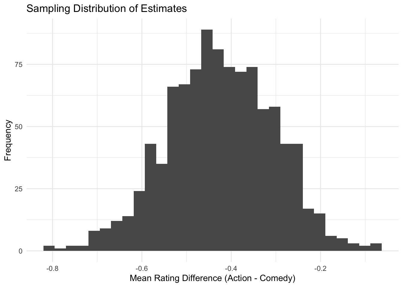

Seems good.

Again, let’s put this into a function

generate_samples <- function(n_simulations, sample_size) {
  
  # Make an empty vector
  estimates <- numeric(n_simulations)
  
  for (i in 1:n_simulations) {
    # Draw a sample with the specified size
    sample <- generate_sample(sample_size) 
    
    # Get an estimate
    estimates[i] <- generate_estimate(sample)
  }
  
  return(estimates)
}

estimates <- generate_samples(n_simulations = 500, sample_size = 500)

ggplot(data.frame(estimates), aes(x = estimates)) +
  geom_histogram() +
  labs(title = "Sampling Distribution of Estimates",
       x = "Mean Rating Difference (Action - Comedy)",
       y = "Frequency") +
  theme_minimal()

`stat_bin()` using `bins = 30`. Pick better value with `binwidth`.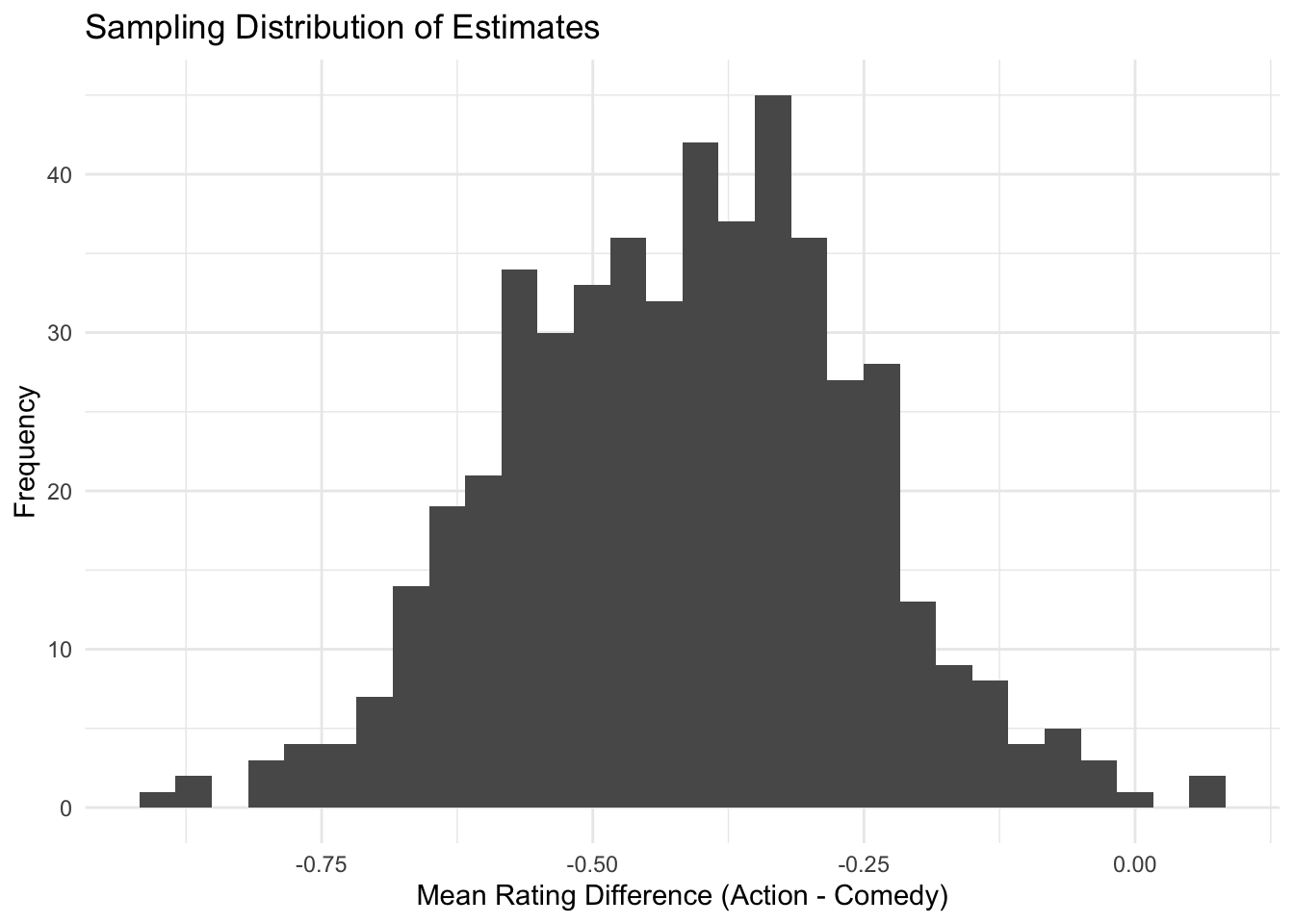

Works fine again.

Step 4: Calculate power

To calculate the power, we first test the statistical significance for each of our 1000 estimates.

To do so, we bring our estimate to the scale of the standard normal distribution and check if it’s smaller than -1.96.

calculate_power <- function(estimates){
  
  # bring on standard normal distribution scale
  estimates_standardized <- estimates/sd(estimates)
  
  # get statistical power 
  power <- data.frame(estimates_standardized) |> 
    mutate(significant = ifelse(estimates_standardized <= -1.96, TRUE, FALSE)) |> 
    summarize(share_significant = sum(significant) / n()) |> 
    pull(share_significant)
  
  return(power)
}

calculate_power(estimates = estimates)

[1] 0.736

Step 5: Bring it all together

We now put all the above functions into a final power_simulation function.

power_simulation <- function(sample_size, n_simulations = 1000) {
  
  # Generate multiple samples and compute estimates
  estimates <- generate_samples(n_simulations, sample_size)
  
  # Calculate statistical power
  power <- calculate_power(estimates)
  
  # Return results
  return(tibble(
    sample_size = sample_size,
    n_simulations = n_simulations,
    estimated_power = power,
    mean_effect = mean(estimates),
    sd_effect = sd(estimates)
  ))
}

Let’s test this function

# run a power simulation for sample size 1000
power_simulation(sample_size = 1000, n_simulations = 1000)

# A tibble: 1 × 5
  sample_size n_simulations estimated_power mean_effect sd_effect
        <dbl>         <dbl>           <dbl>       <dbl>     <dbl>
1        1000          1000           0.935      -0.422     0.121

🎉 Seems to have worked just fine.

Step 6: Repeat the whole process

We write a for loop, for different sample sizes we would like to test. Remember that the output of our power_data() function is a data frame, so we initialize an empty data frame where we can store the results of all iterations.

Note that running the code chunk below takes a couple of seconds.

sample_sizes <- c(50, 100, 500, 1000)

# make an empty data frame
power_data <- tibble()

for (i in sample_sizes) {
  # run power simulation
  power <- power_simulation(sample_size = i, n_simulations = 1000)
  
  power_data <- bind_rows(power_data, power)
}

power_data

# A tibble: 4 × 5
  sample_size n_simulations estimated_power mean_effect sd_effect
        <dbl>         <dbl>           <dbl>       <dbl>     <dbl>
1          50          1000           0.127      -0.432     0.518
2         100          1000           0.208      -0.423     0.371
3         500          1000           0.751      -0.436     0.169
4        1000          1000           0.971      -0.431     0.111

🎉 Worked!

We can plot the results.

ggplot(power_data, 
       aes(x = sample_size, y = estimated_power)) +
  geom_line(color = 'red', size = 1.5) + 
  # add a horizontal line at 80%
  geom_hline(aes(yintercept = .8), linetype = 'dashed') + 
  # Prettify!
  theme_minimal() + 
  scale_y_continuous(labels = scales::percent, limits = c(0,1)) + 
  labs(title = "Power Simulation for a difference of -0.5 between action and comedy movies",
       x = 'Sample Size', y = 'Power')

Warning: Using `size` aesthetic for lines was deprecated in ggplot2 3.4.0.
ℹ Please use `linewidth` instead.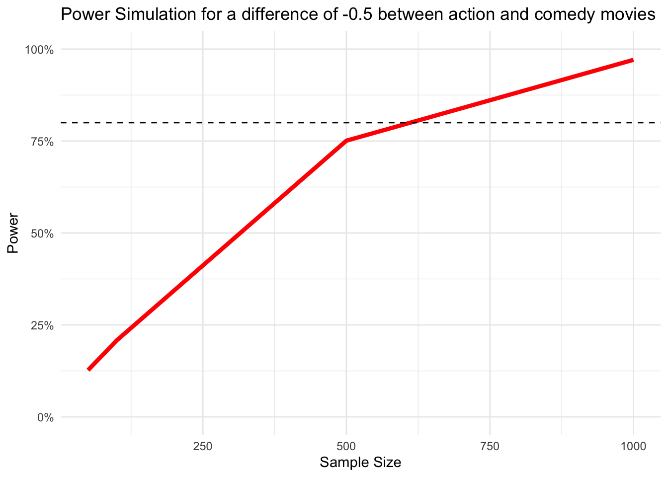

From the curve, we can read that we reach our desired power level somewhere between a sample size of 500 and 1000, but a lot closer to 500.