Abstract

In recent years, many studies have proposed individual-level interventions to reduce people’s susceptibility for believing in misinformation. However, the results are often not directly comparable, because researchers have used different modes of evaluating the effectiveness of these interventions. Here, we will re-assess the findings of this literature in a Signal Detection Theory (SDT) framework. This allows us to differentiate between two different kinds of intervention effects: First, the effect on sensitivity, which is the ability of discriminating between true and false news that researchers typically look for. Second, the effect on response bias, which is the extent to which participants become generally more/less skeptical in their accuracy ratings for all news (whether true or false). We will run an Individual Participant Data (IPD) meta-analysis based on a sample of studies that we identified via a systematic literature review following the PRISMA guidelines. We will use a two-stage approach: First, we extract individual participant data and run a Signal Detection Theory analysis separately for each experiment. Second, we will run a meta-analysis on the experiment-level outcomes.

Code

# load plot theme
source("../R/plot_theme.R") 

# load other functions
source("../R/custom_functions.R")

Note

This preregistration has been registered on the OSF on December 2, 2024.

Introduction

In recent years, many studies have tested interventions designed to help people detect online misinformation. However, the results are often not directly comparable, because researchers have used different modes of evaluating the effectiveness of these interventions (Guay et al. 2023). Moreover, the most popular outcome measure–a discernment score based on Likert-scale mean differences between true and false news–has recently been shown to be biased (Higham, Modirrousta-Galian, and Seabrooke 2024).

The aim of this study re-analyze these studies in a common framework to draw new conclusions about the effectiveness of individual-level interventions designed to reduce people’s susceptibility for believing in misinformation. Following a recent literature (Higham, Modirrousta-Galian, and Seabrooke 2024; Gawronski, Nahon, and Ng 2024; Modirrousta-Galian and Higham 2023; Batailler et al. 2019) we will use a Signal Detection Theory (SDT) framework. This allows us to evaluate two different effects of interventions: First, the effect on sensitivity, which is the ability of discriminating between true and false news. Second, the effect on response bias, which is the extent to which participants shift their general response criterion, i.e. the extent to which they become generally more/less skeptical in their accuracy ratings for all news (regardless of whether true or false).

We formulate two main research questions: How do interventions against misinformation affect: (i) people’s ability to discriminate between true and false news (sensitivity, or “d’”, in a SDT framework; RQ1)?, and (ii) people’s skepticism towards news in general (i.e. response bias, or “c”, in a SDT framework; RQ2)?

We will also test some moderator effects. At this stage, we know that we will ask the following questions: Do the effects of the interventions (both on sensitivity and response bias) differ between (i) different types of interventions; (ii) politically concordant and politically discordant news; (iii) different age groups? It is likely that after data collection, we will have a better overview of variables and would want to ask more moderator questions. If that is the case, we will specify these moderators in a second pre-registration before analysis.

We will do an Individual Participant Data meta-analysis (IPD), using a two-stage approach: First, we extract individual participant data from relevant studies and run a Signal Detection Theory analysis separately for each experiment. Second, we run a meta-analysis on the outcomes of the experiments.

Methods

Data/Sampling

Systematic Literature review

We will base ourselves on the systematic literature review of a recent meta-analysis on people’s accuracy judgments of true and false news (Pfänder and Altay 2024). Of all the studies extracted from this review, we will reduce our sample to those that tested an intervention to augment news discernment.

Since the field is rapidly growing, we will also try to add papers that have been published since the systematic review. We will code for all papers whether they were part of the original systematic review of Pfänder and Altay (2024) or identified afterwards, so that the selection process is transparent. In a second pre-registration–after data collection but before analysis–we will publish a full list of studies, detailing whether they were part of the systematic review or added afterwards by us because we came across them.

We have already stored individual level data for several studies used in Pfänder and Altay (2024). We have yet to collect data for the remaining studies. For the studies for which we already have stored individual-level data, we have not yet cleaned it according to the requirements of the study proposed here. We have not performed any of the here suggested analysis on the collected data. We have simulated data to be clear on the data structure our analysis requires and to test how well our model performs in recovering parameters. All analyses presented in this pre-registration use this simulated data.

Selecting Interventions

Sometimes, within the same experiment, researchers test different interventions, by comparing it to a single control group. For a meta-analysis, this is a problem, sometimes referred to as double-counting. Dependencies between effect sizes based on the same comparison group cannot be accounted for by a meta-analytic model (Harrer et al. 2021). As a consequence, we will have to make a selection of for experiments that test several interventions at the same time: Following options recommended in the cochrane manual we use the following rule of thumb: If the interventions are conceptually similar enough, pool the interventions together. If they are too dissimilar, pick the most pertinent one.

It is hard to predict in advance how relevant these decisions will be. However, we will make them on a purely theoretical basis: Once we have collected our data, we will make an overview of all interventions, and make a decision in case of multiple intervention arms within the same experiment. We will preregister these decisions as part of the second pre-registration. Only then will we run the analysis.

We have tried to mimic the situation of multiple intervention groups but only one control group in our simulated data. Some experiments have several interventions, and they are sometimes conceptually similar, sometimes different. Table 1 shows the experimental structure of the first two simulated papers.

Code

data %>% 
  filter(paper_id %in% c(1:2)) %>% 
  distinct(paper_id, experiment_id, intervention_id, intervention_type) %>% 
  kable(caption = "Experimental structure of the first two simulated papers",
        booktabs = TRUE) %>% 
    kable_styling(font_size = 10)

Table 1: Experimental structure of the first two simulated papers

paper_id	experiment_id	intervention_id	intervention_type
1	1	NA	control
1	1	1	priming
1	2	NA	control
1	2	1	warning labels
2	1	NA	control
2	1	1	priming
2	1	2	warning labels
2	2	NA	control
2	2	1	warning labels

In Paper 1, there are two experiments (experiment_id = ‘1’ and experiment_id = ‘2’). Both experiments only have two arms, respectively: the control group and an intervention group (priming for Experiment 1; warning labels for Experiment 2). In these cases, since there is only one intervention, there is no decision to make as to which intervention to keep. By contrast, the first experiment of Paper 2 has three arms, among with two different intervention types (‘priming’ and ‘warning labels’). In such a case, we would need to make a decision on which intervention type to keep. This decision will probably depend on which intervention type occurred how many times etc.

In our data, we will first detect all experiments with multiple interventions (Table 2).

Code

conflict <- data %>% 
  distinct(paper_id, experiment_id, unique_experiment_id, intervention_id, intervention_type) %>% 
  group_by(unique_experiment_id) %>% 
  # substact 1 because of the control condition
  summarize(n_different_intervention_types = n_distinct(intervention_type) - 1, 
            # display different intervention types
            types = paste(unique(intervention_type), collapse = ", ")
            ) %>% 
  # label all experiments with more than one intervention type
  mutate(conflict = ifelse(n_different_intervention_types > 1, TRUE, FALSE)) %>% 
  filter(conflict == TRUE)

conflict %>% 
  kable(caption = "Studies with mutliple intervention arms in the simulated data", 
        booktabs = TRUE) %>% 
    kable_styling(font_size = 10)

Table 2: Studies with mutliple intervention arms in the simulated data

unique_experiment_id	n_different_intervention_types	types	conflict
10_2	2	control, priming, literacy tips	TRUE
10_3	2	control, priming, warning labels	TRUE
2_1	2	control, priming, warning labels	TRUE
3_1	2	control, warning labels, literacy tips	TRUE
4_1	2	control, literacy tips, priming	TRUE
5_1	2	control, warning labels, priming	TRUE
6_1	2	control, literacy tips, priming	TRUE
6_2	2	control, warning labels, literacy tips	TRUE
7_1	2	control, literacy tips, priming	TRUE
7_3	2	control, priming, literacy tips	TRUE
8_1	2	control, warning labels, priming	TRUE
9_1	2	control, warning labels, priming	TRUE
9_2	2	control, literacy tips, priming	TRUE

We will then have to make specific exclusion decisions for each experiment (Table 3).

Code

conflict <- conflict %>% 
  # list all intervention types to be excluded for a given experiment
  mutate(exclude =   case_when(unique_experiment_id == "1_1" ~ "priming, warning labels",
                               unique_experiment_id == "10_1" ~ "priming",
                               unique_experiment_id == "10_3" ~ "warning labels",
                               # continue this list for all studies (we don't do this here because lazy)
                               TRUE ~ NA_character_
  )
  ) %>% 
  select(unique_experiment_id, exclude)

conflict %>% 
  kable(caption = "Example of exclusion decisions for some of the experiments with multiple intervention arms", 
        booktabs = TRUE) %>% 
    kable_styling(font_size = 10)

Table 3: Example of exclusion decisions for some of the experiments with multiple intervention arms

unique_experiment_id	exclude
10_2	NA
10_3	warning labels
2_1	NA
3_1	NA
4_1	NA
5_1	NA
6_1	NA
6_2	NA
7_1	NA
7_3	NA
8_1	NA
9_1	NA
9_2	NA

We then filter our data to only keep the intervention conditions we decided upon (Table 4).

Table 4

Code

data <- data %>% 
  left_join(conflict) %>% 
  # Use str_detect to check if intervention_type is found in exclude string
  filter(is.na(exclude) | !str_detect(exclude, intervention_type))

# check
# data %>%
#   distinct(paper_id, experiment_id, unique_experiment_id, intervention_id, intervention_type, condition) %>%
#   filter(unique_experiment_id %in% c("10_1", "2_1", "5_1"))

Once all decisions regarding the intervention selections have been made, we can rely our ‘condition’ variable for all models below, which takes only the values of either ‘control’ or ‘intervention’.

Analysis plan

Outcomes

We want to measure the effects of misinformation interventions on two outcomes of Signal Detection Theory (SDT): \(d'\) (“d prime”, sensitivity), and \(c\) (response bias). Table 5 shows how instances of news ratings map onto SDT terminology.

Code

# Data
table_data <- tibble(
  Stimulus = c("True news (target)","False news (distractor)"),
  Accurate = c("Hit", "False alarm"),
  `Not Accurate` = c("Miss", "Correct rejection")
)

# Set Stimulus as row names
# rownames(table_data) <- table_data$Stimulus
# table_data$Stimulus <- NULL

# Create table using kable
kable(table_data, 
      caption = "Accuracy ratings in Signal Detection Theory terms", 
              booktabs = TRUE) %>%
  kable_paper(full_width = FALSE) %>%
  add_header_above(c(" ", "Response" = 2))

Table 5: Accuracy ratings in Signal Detection Theory terms

	Response
Stimulus	Accurate	Not Accurate
True news (target)	Hit	Miss
False news (distractor)	False alarm	Correct rejection

Code

# make SDT variables
sdt_data <- data %>% 
  # code ratings in terms of SDT language
  mutate(sdt_outcome = case_when(accuracy == 1 & veracity == "true" ~ "hit", 
                                 accuracy == 1 & veracity == "fake" ~ "false_alarm",
                                 accuracy == 0 & veracity == "true" ~ "miss",
                                 accuracy == 0 & veracity == "fake" ~ "correct_rejection",
                                 .default =  NA)
         )

The sensitivity, \(d’\), measures people’s capacity to discriminate between true and false news. It is defined as the difference of the standardized hit and false alarm rates

\[ d' = \Phi^{-1}(HR) - \Phi^{-1}(FAR) \]

where \(HR\) refers to hit rate or the proportion of true news trials that participants classified–correctly–as “accurate” (\(HR = \frac{N_{Hits}}{N_{Hits} + N_{Misses}}\)), \(FAR\) refers to false alarm rate or the proportion of false news trials that participants classified–incorrectly–as “accurate” (\(HR = \frac{N_{False Alarms}}{N_{FalseAlarms} + N_{Correct Rejections}}\)). \(\Phi\) is the cumulative normal density function, and is used to convert z scores into probabilities. Its inverse, \(\Phi^{-1}\), converts a proportion (such as a hit rate or false alarm rate) into a z score. Below, we refer to standardized hit and false alarm rates as zHR and zFAR, respectively. Due to this transformation, a proportion of .5 is converted to a z score of 0 (reflecting responses at chance). Proportions greater than .5 produce positive z scores, and proportions smaller than .5 negative ones. A positive \(d'\) score indicates that people rate true news as more accurate than false news.

The response bias, \(c\) can be conceived of as an overall tendency to rate items as accurate. It is defined as

\[ c = -\frac{1}{2}(\text{zHR} + \text{zFAR}) \]

Note that \(c\) = 0 when \(zFAR = -zHR\). Because \(-zHR = z(1-HR)\) is the (z-transformed) share of misses (true news rated as “not accurate”), \(c\) = 0 when the false alarm rate is equal to the rate of misses (Macmillan & Creelman (2004). In other words, if people–mistakenly–rate true news as not accurate (the rate of misses) as much as they–mistakenly–rate false false news as accurate (the rate of false alarms), then there is no response bias. A positive \(c\) score occurs when the miss rate (rating true news news as false) is larger than the false alarm rate (rating false news as true). In other words, a positive \(c\) score indicates that people were more skeptical towards true news than they were gullible towards false news. We refer to this as an overall tendency towards skepticism.

Our outcomes of interest are the intervention effects on \(d'\) (“d prime”, sensitivity) and \(c\) (response bias). Since these outcomes are about the difference between the control and the treatment group, we call them “Delta”. Specifically, they are defined as:

\[ \Delta d' = d'_{treatment} - d'_{control} \]

and

\[ \Delta c = c_{treatment} - c_{control}. \]

A positive \(\Delta d'\) score indicates that the intervention increased participants’ ability to discriminate between true and false news compared to the control group. A positive \(\Delta c\) score indicates that the intervention led to a greater tendency towards skepticism, meaning participants were more likely to rate items as “not accurate” regardless of veracity, compared to the control group.

Variables

Table 6 contains a list of variables we will collect. We might not be able to collect all variables for all studies. For political concordance, e.g., this will certainly not be the case.

Code

# Create the codebook data frame
codebook <- data.frame(
  Variable_Name = c(
    "paper_id", "experiment_id", "subject_id", "country", "year", 
    "veracity", "condition", "intervention_label", "intervention_description", 
    "intervention_selection",
    "accuracy_raw", "scale", "originally_identified_treatment_effect", 
    "concordance", "age", "age_range", "identified_via", "id", 
    "unique_experiment_id", "accuracy"
  ),
  Description = c(
    "Identifier for each paper",
    "Identifier for each experiment within a paper",
    "Identifier of individual participants within an experiment",
    "The country of the sample",
    "Ideally year of data collection, otherwise year of publication",
    "Identifying false and true news items",
    "Treatment vs. control",
    "A label for what the intervention consisted of",
    "A detailed description of the intervention",
    "If multiple interventions tested within a single experiment (and related to a single control group), reasoning as to which intervention to select",
    "Participants' accuracy ratings on the scale used in the original study",
    "The scale used in the original study",
    "Whether the authors identified a significant treatment effect (`FALSE` if no, `TRUE` if yes)",
    "Political concordance of news items (concordant or discordant)",
    "Participant age. In some cases, participant age will not be exact, but within a binned category. In this case, we will take the mid-point of this category for the age variable",
    "Binned age, if only this is provided by the study.",
    "Indicates if a paper was identified by the systematic review or added after",
    "Unique participant ID (merged `paper_id`, `experiment_id`, `subject_id`)",
    "Unique experiment ID (merged `paper_id` and `experiment_id`)",
    "Binary version of `accuracy_raw`; unchanged if originally binary"
  )
)

# Generate the styled table with kableExtra
kable(codebook, 
      caption = "Codebook for variables to collect",
      col.names = c("Variable Name", "Description"),
      booktabs = TRUE,
      longtable = TRUE,) %>%
  kable_styling(latex_options = "repeat_header",
                font_size = 10) %>% 
  column_spec(1, bold = TRUE) %>%  # Bold the first column
  column_spec(2, width = "25em") %>%  # Set width for the description column
  row_spec(0, bold = TRUE)  # Bold the header row

Table 6: Codebook for variables to collect

Variable Name	Description
paper_id	Identifier for each paper
experiment_id	Identifier for each experiment within a paper
subject_id	Identifier of individual participants within an experiment
country	The country of the sample
year	Ideally year of data collection, otherwise year of publication
veracity	Identifying false and true news items
condition	Treatment vs. control
intervention_label	A label for what the intervention consisted of
intervention_description	A detailed description of the intervention
intervention_selection	If multiple interventions tested within a single experiment (and related to a single control group), reasoning as to which intervention to select
accuracy_raw	Participants' accuracy ratings on the scale used in the original study
scale	The scale used in the original study
originally_identified_treatment_effect	Whether the authors identified a significant treatment effect (`FALSE` if no, `TRUE` if yes)
concordance	Political concordance of news items (concordant or discordant)
age	Participant age. In some cases, participant age will not be exact, but within a binned category. In this case, we will take the mid-point of this category for the age variable
age_range	Binned age, if only this is provided by the study.
identified_via	Indicates if a paper was identified by the systematic review or added after
id	Unique participant ID (merged `paper_id`, `experiment_id`, `subject_id`)
unique_experiment_id	Unique experiment ID (merged `paper_id` and `experiment_id`)
accuracy	Binary version of `accuracy_raw`; unchanged if originally binary

Building a comparable accuracy measure that we can analyze in the SDT framework outlined here, requires collapsing scales. The studies that we will look at use a variety of scales. Some use a binary scale, which is the one that is the most straightforward to use in a SDT framework (signal vs. no signal) and thus also the one we have simulated. However, a lot of studies use Likert-type scales. For these studies, we will collapse the original scores into a dichotomized version with answers of either ‘not accurate’ (0) or ‘accurate’ (1). For example, a study might have used a 4-point scale going from 1, not accurate at all, to 4, completely accurate. In this case, we will code responses of 1 and 2 as not accurate (0) and 3 and 4 as accurate (1). For scales, with a mid-point (example 3 on a 5-point scale), we will code midpoint answers as ‘NA’, meaning they will be excluded from the analysis.

Main Analysis

We will run a participant-level meta analysis using a two-stage approach: First, for each experiment, we calculate a generalized linear mixed model (glmm) that yields SDT outcomes. The resulting estimates are our effect sizes. Second, we run a meta analysis on these effect sizes. In Appendix Section 6.1 to this registration, we explain step by step how to go from a by-hand SDT analysis to a glmm SDT analysis. In the following, we will outline the analysis steps we will perform.

Stage 1: experiment-level analysis

For each experiment, we run a separate participant-level SDT analysis. Because participants provide several ratings, we use mixed-models with random participant effects that account for the resulting dependency in the data points. We use random effects both for the intercept and the effect of veracity. We do not use random effects for condition or the interaction of condition and veracity, as condition is typically manipulated between participants. We can obtain SDT outcomes directly from a generalized linear mixed model (glmm) when using a probit link function (see Appendix Section 6.1). Table 7 shows the model output for our simulated Experiment 1, from paper 1.

Code

# calculate model function
calculate_model <- function(data) {
  
  time <- system.time({
    model <- glmer(accuracy ~ veracity_numeric + condition_numeric + 
                     veracity_numeric*condition_numeric +
                     (1 + veracity_numeric | unique_subject_id),
                   data = data, 
                   family = binomial(link = "probit")
    )
  })
  
  time <- round(time[3]/60, digits = 2)
  
  # get a tidy version
  model <- tidy(model, conf.int = TRUE) %>% 
    # add time
    mutate(time_minutes = time)
  
  return(model)
  
}
# test
# mixed_model <- calculate_model(data %>% filter(unique_experiment_id == "1_1"))
# mixed_model

We calculate one model per experiment and store the results in a common data frame.

Code

# Running this model takes some time. We therefor stored the results in a data frame that we can reload. 
filename <- "../data/simulations/models_by_experiment.csv" 

run_loop <- function(data, filename){
  
  # only execute the following if the file does NOT exist
  if (!file.exists(filename)) {
    
    # make a vector with all unique experiment ids
    experiments <- data %>% 
      distinct(unique_experiment_id) %>% 
      # slice(1:3) %>% # to test loop
      pull()
    
    time <- system.time({
      
      # run one model per experiment and store the results in a common data frame
      results <- experiments %>%
        map_dfr(function(x) {
          
          # restrict data to only the respective experiment
          experiment <- data %>% filter(unique_experiment_id == x)
          
          # extract paper id
          paper_id <- unique(experiment$paper_id)
          
          # To keep track of progress
          print(paste("calculating model for experiment ", x))
          
          model_experiment <- calculate_model(experiment) %>%
            mutate(unique_experiment_id = x,
                   paper_id = paper_id)
          
          return(model_experiment)
        })
    })
    
    write_csv(results, filename)
    
    print(paste("Elapsed time: ", round(time[3]/60, digits = 2), " minutes"))
  }
  
}

# execute function
run_loop(data, filename)

# read saved model results
model_results <- read_csv(filename)

We code our binary independent variables, veracity and condition, using deviation coding (i.e. for veracity, false = -0.5, true = 0.5; for condition, control = -0.5, treatment = 0.5). Using deviation coding, the main effect model output terms translate to SDT outcomes as follows:

(Intercept) = average -\(c\), pooled across all conditions
veracity_numeric = average \(d'\), pooled across all conditions
condition_numeric = -\(\Delta c\), i.e. the change in -response bias between control and treatment
veracity_numeric:condition_numeric = \(\Delta d'\), i.e. the change in sensitivity between control and treatment

Code

# We clean up the model output by naming our estimates of interest in terms of SDT outcomes, and reversing the coefficients for response bias c, and delta response bias c.

model_results <- model_results %>% 
  filter(effect == "fixed") %>% 
  mutate(
    # make sdt outcomes
    SDT_term = case_when(
    term == "(Intercept)" ~ "average c",
    term == "veracity_numeric" ~ "average d'",
    term == "condition_numeric" ~ "delta c",
    term == "veracity_numeric:condition_numeric" ~ "delta d'",
    TRUE ~ "Other"
  ), 
  # reverse c and delta c estimates
  SDT_estimate = ifelse(term == "(Intercept)" | term == "condition_numeric", 
                        -1*estimate, estimate),
    sampling_variance = std.error^2
  )

Code

model_results %>% 
  filter(unique_experiment_id == "1_1") %>% 
  select(-starts_with("conf")) %>% 
  rounded_numbers() %>% 
  select(-c(effect, group)) %>% 
  kable(
    caption = "Results of a generalize linear mixed model (glmm)",
    booktabs = TRUE) %>%
  kable_styling(font_size = 8,  # Set a smaller font size
                latex_options = c("scale_down")) # Scale down the table

Table 7: Results of a generalize linear mixed model (glmm)

term	estimate	std.error	statistic	p.value	time_minutes	unique_experiment_id	paper_id	SDT_term	SDT_estimate	sampling_variance
(Intercept)	-0.514	0.032	-16.175	0.000	0.01	1_1	1	average c	0.514	0.001
veracity_numeric	0.786	0.062	12.711	0.000	0.01	1_1	1	average d'	0.786	0.004
condition_numeric	-0.119	0.063	-1.892	0.059	0.01	1_1	1	delta c	0.119	0.004
veracity_numeric:condition_numeric	-0.285	0.123	-2.312	0.021	0.01	1_1	1	delta d'	-0.285	0.015

As shown in Figure 1, we can then plot the distributions of our outcome estimates of interest, across experiments.

Code

# make plot
ggplot(model_results, aes(x = estimate, fill = SDT_term)) +
  geom_density(alpha = 0.5, adjust = 1.5) +
  # colors 
  scale_fill_viridis_d(option = "inferno", begin = 0.1, end = 0.9) +
  # labels and scales
  labs(x = "z-Score", y = "Density") +
  guides(fill = FALSE, color = FALSE) +
  plot_theme +
  theme(strip.text = element_text(size = 14)) +
  facet_wrap(~SDT_term)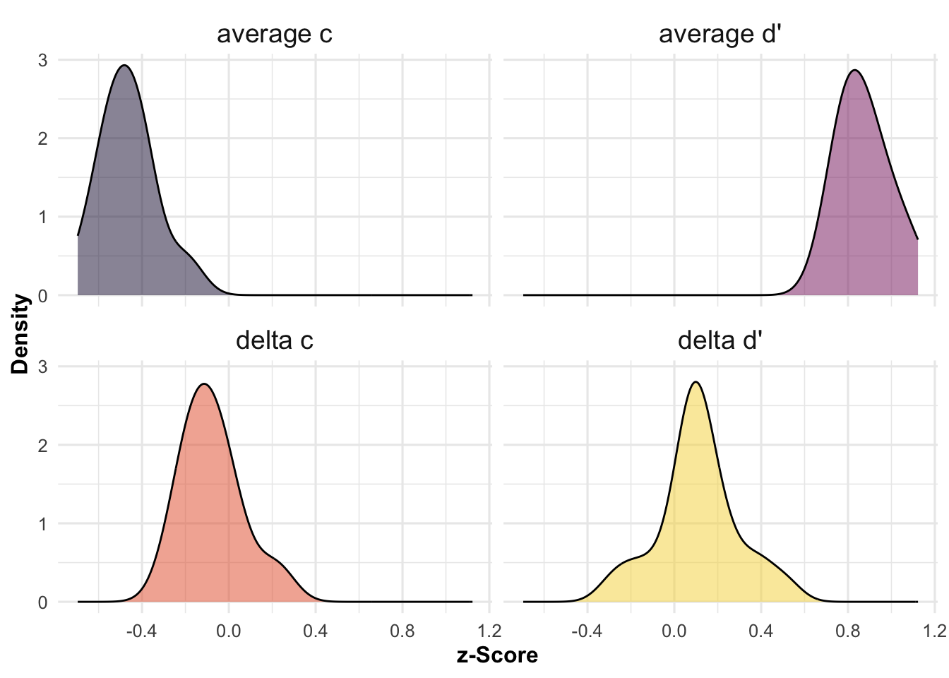

Figure 1: Distributions of Signal Detection Theory outcomes across experiments. Note that these distributions are purely descriptive - effect sizes are not weighted by sample size of the respective experiment, as they are in the meta-analysis.

Stage 2: Meta-analysis

Next, we run a meta analysis on these effect size estimates at the experiment-level. In our models for the meta analysis, each effect size is weighted by the inverse of its standard error, thereby giving more weight to experiments with larger sample sizes. We will use random effects models, which assume that there is not only one true effect size but a distribution of true effect sizes. We will use a multi-level meta-analytic model, with random effects at the publication and the experiment level. This approach allows us to account for the hierarchical structure of our data, in which (at least some) papers (level three) contribute several effect sizes from different experiments (level two)¹. However, the multi-level models do not account for dependencies in sampling error. When one paper contributes several effect sizes, one might expect their respective sampling errors to be correlated. To account for dependency in sampling errors, we compute cluster-robust standard errors, confidence intervals, and statistical tests for all meta-analytic estimates. For our simulated data, Table 8 shows the results of the meta-analytic models and Figure 2 provides an overview of effect sizes for each experiment as a forest plot.

Code

# Function to calculate meta models
calculate_models <- function(data, yi, vi, robust = TRUE) {
  
  # provide metafor compatible names
  metafor_data <- data %>% 
    rename(yi = {{yi}}, 
           vi = {{vi}})
  
  # Multilevel random effect model for accuracy
  model <-  metafor::rma.mv(yi, vi, random = ~ 1 | paper_id / unique_experiment_id, 
                            data = metafor_data)
  
  return(model)
  
  if(robust == TRUE) {
    # with robust standard errors clustered at the paper level 
    robust_model <- robust(model, cluster = data$paper_id)
    
    return(robust_model)
  }
}

Code

# model for delta dprime
delta_dprime <- calculate_models(data = model_results %>% 
                                   filter(SDT_term == "delta d'"), yi = SDT_estimate, 
                                 vi = sampling_variance, robust = TRUE)

# model for delta c
delta_c <- calculate_models(data = model_results %>% 
                                   filter(SDT_term == "delta c"), yi = SDT_estimate, 
                                 vi = sampling_variance, robust = TRUE)


modelsummary::modelsummary(list("Delta d'" = delta_dprime, 
                                "Delta c" = delta_c
                                ), 
                           title = "Results of Meta-analysis",
                           stars = TRUE, 
                           output = "kableExtra"
                           )

Table 8: Results of Meta-analysis

	Delta d'	Delta c
overall	0.100*	0.078*
	(0.043)	(0.032)
Num.Obs.	21	21
AIC	−8.1	−20.4
BIC	−4.9	−17.3
+ p < 0.1, * p < 0.05, p < 0.01, * p < 0.001

Code

# Set up a 1x2 layout for the two plots
par(mfrow = c(1, 2))

# Calculate weights (e.g., inverse of standard error)
model_results <- model_results %>%
  mutate(weight = 1 / sqrt(sampling_variance))

# Create plot for d'
forest.rma(delta_dprime,
           xlim = c(-1, 2),          # Adjust horizontal plot region limits
           at = c(-1, -0.5, 0, 1, 2), 
           order = "obs",            # Order by size of yi
           slab = unique_experiment_id, 
           annotate = TRUE,          # Study labels and annotations
           efac = c(0, 1),           # Remove vertical bars at end of CIs
           pch = 15,                 # Change point symbol to filled squares
           col = "gray40",           # Change color of points/CIs
           cex.lab = 0.8, 
           cex.axis = 0.8,           # Increase size of x-axis title/labels
           lty = c("solid", "dotted", "blank"),  # Remove horizontal line at top of plot
           mlab = "BLASt", 
           ylim = c(-2, n_distinct(model_results$unique_experiment_id)), 
           addfit = FALSE, 
           xlab = "Delta d'") 
addpoly(delta_dprime, mlab = " ", cex = 1, row = -2) 
abline(h = 0)

# Create plot for c
forest.rma(delta_c,
           xlim = c(-1, 2),          # Adjust horizontal plot region limits
           at = c(-1, -0.5, 0, 1, 2), 
           order = "obs",            # Order by size of yi
           slab = unique_experiment_id, 
           annotate = TRUE,          # Study labels and annotations
           efac = c(0, 1),           # Remove vertical bars at end of CIs
           pch = 15,                 # Change point symbol to filled squares
           col = "gray40",           # Change color of points/CIs
           cex.lab = 0.8, 
           cex.axis = 0.8,           # Increase size of x-axis title/labels
           lty = c("solid", "dotted", "blank"),  # Remove horizontal line at top of plot
           mlab = "BLASt", 
           ylim = c(-2, n_distinct(model_results$unique_experiment_id)), 
           addfit = FALSE, 
           xlab = "Delta c") 
addpoly(delta_c, mlab = " ", cex = 1, row = -2) 
abline(h = 0)

# Reset the layout to the default (1x1)
par(mfrow = c(1, 1))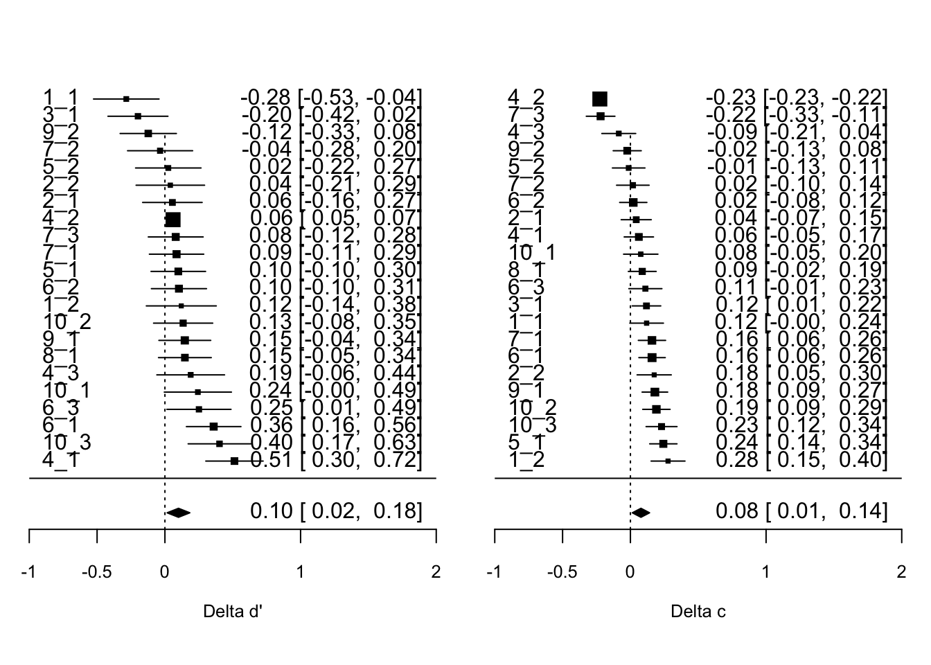

Figure 2: *Forest plots for delta d’ and delta c*. The figure displays all effect sizes for both outcomes. Effects are weighed by their sample size. Effect sizes are z-values. Horizontal bars represent 95% confidence intervals. The average estimate is the result of a multilevel meta model with clustered standard errors at the sample level.

Moderator analysis

We distinguish between two broad kinds of moderator variables: those that vary within-experiments (e.g. political concordance) and those that vary between experiments (e.g. intervention type). We will use different approaches for these two kinds.

a. within-experiment variables

There are two moderator variables that vary within-experiments that we will test: age and political concordance. Age varies within experiments, but between participants (each participant can only have one age). Political concordance varies not only within experiments, and also within participants–in the typical experiment design, each participant is shown both concordant and discordant items. In the follwing, we will focus on political concordance, which requires slightly more complex modelling, but provide the models for age in the respective code chunks².

We have two options: The first is integrating political concordance in our baseline model. While this would be the straightforward thing to do, it involves a three-way interaction with many random effects and will likely bring up convergence issues. The second option is to run our baseline model separately for concordant and discordant items, and then proceed as for between-experiment moderators. We will try the first option first, and only revert to the second if we encounter serious convergence issues.

i. Integrating Concordance in baseline model

In the first option, we add political concordance to our Stage 1 model, such that we have a three-way interaction between veracity, condition and political concordance.

Code

# calculate model function for political concordance
calculate_concordance_model <- function(data) {
  
  time <- system.time({
    model <- glmer(accuracy ~ veracity_numeric + condition_numeric + concordance_numeric + 
                     veracity_numeric*condition_numeric*concordance_numeric +
                     (1 + veracity_numeric + veracity_numeric:concordance_numeric | 
                        unique_subject_id),
                   data = data, 
                   family = binomial(link = "probit")
    )
  })
  
  time <- round(time[3]/60, digits = 2)
  
  # get a tidy version
  model <- tidy(model, conf.int = TRUE) %>% 
    # add time
    mutate(time_minutes = time)
  
  return(model)
  
}

# calculate model function for age
calculate_age_model <- function(data) {
  
  time <- system.time({
    model <- glmer(accuracy ~ veracity_numeric + condition_numeric + age + 
                     veracity_numeric*condition_numeric*age +
                     (1 + veracity_numeric  | 
                        unique_subject_id),
                   data = data, 
                   family = binomial(link = "probit")
    )
  })
  
  time <- round(time[3]/60, digits = 2)
  
  # get a tidy version
  model <- tidy(model, conf.int = TRUE) %>% 
    # add time
    mutate(time_minutes = time)
  
  return(model)
  
}
# age_model <- calculate_age_model(data %>% filter(unique_experiment_id == "1_1"))
# age_model %>% print(n = 14)

Table 9 illustrates the model output for the first experiment (Experiment 1 of Paper 1) in our simulated data.

Code

concordance_model <- calculate_concordance_model(data %>% filter(unique_experiment_id == "1_1"))
concordance_model %>% 
  rounded_numbers() %>% 
  select(-c(effect, group)) %>% 
  kable(booktabs = TRUE, 
        caption = "Results of the generalized linear mixed model (glmm) on the first experiment (Experiment 1 of Paper 1) in our simulated data.") %>%
  kable_styling(font_size = 8,  # Set a smaller font size
                latex_options = c("scale_down")) # Scale down the table

Table 9: Results of the generalized linear mixed model (glmm) on the first experiment (Experiment 1 of Paper 1) in our simulated data.

term	estimate	std.error	statistic	p.value	conf.low	conf.high	time_minutes
(Intercept)	-0.510	0.033	-15.511	0.000	-0.574	-0.445	0.05
veracity_numeric	0.808	0.063	12.740	0.000	0.684	0.933	0.05
condition_numeric	-0.112	0.065	-1.723	0.085	-0.239	0.015	0.05
concordance_numeric	-0.095	0.063	-1.504	0.133	-0.219	0.029	0.05
veracity_numeric:condition_numeric	-0.287	0.126	-2.283	0.022	-0.534	-0.041	0.05
veracity_numeric:concordance_numeric	-0.181	0.129	-1.400	0.161	-0.435	0.072	0.05
condition_numeric:concordance_numeric	-0.009	0.125	-0.074	0.941	-0.255	0.236	0.05
veracity_numeric:condition_numeric:concordance_numeric	-0.197	0.255	-0.770	0.441	-0.697	0.304	0.05
sd__(Intercept)	0.119	NA	NA	NA	NA	NA	0.05
cor__(Intercept).veracity_numeric	1.000	NA	NA	NA	NA	NA	0.05
cor__(Intercept).veracity_numeric:concordance_numeric	1.000	NA	NA	NA	NA	NA	0.05
sd__veracity_numeric	0.085	NA	NA	NA	NA	NA	0.05
cor__veracity_numeric.veracity_numeric:concordance_numeric	1.000	NA	NA	NA	NA	NA	0.05
sd__veracity_numeric:concordance_numeric	0.342	NA	NA	NA	NA	NA	0.05

Given that all our binary variables in the data are deviation-coded (-0.5 vs. 0.5) outputs are to be interpreted as follows:

(Intercept) = average -\(c\), pooled across all conditions
veracity_numeric = average \(d'\), pooled across all conditions
condition_numeric = -\(\Delta c_{\text{condition}}\), i.e. the change in -response bias between control and treatment, pooled across concordant and discordant items
concordance_numeric = -\(\Delta c_{\text{concordance}}\), i.e. the change in -response bias between concordant and discordant items, pooled across control and treatment
veracity_numeric:condition_numeric = \(\Delta d'_{\text{condition}}\), i.e. the change in sensitivity between control and treatment, pooled across concordant and discordant items
veracity_numeric:concordance_numeric = \(\Delta d'_{\text{concordance}}\), i.e. the change in sensitivity between concordant and discordant items, pooled across control and treatment
condition_numeric:concordance_numeric = Effect of concordance on -\(\Delta c_{\text{condition}}\),
veracity_numeric:condition_numeric:concordance_numeric = Effect of concordance on \(\Delta d'_{\text{condition}}\)

Since interpretation can get a bit complex in three-way interactions here is a good ressource, we demonstrate below that the model estimates correspond to their respective SDT outcomes.

To do so, we first run the same model as before, on the same data as before (Experiment 1 of Paper 1), but removing the random effects, so that our model estimates will correspond to the estimates from a by-hand Signal Detection Theory analysis (Table 10).

Code

# same model as above, but without random effects 
glm_model <- glm(accuracy ~ veracity_numeric + condition_numeric + concordance_numeric + 
                     veracity_numeric*condition_numeric*concordance_numeric,
                   data = data %>% filter(unique_experiment_id == "1_1"), 
                   family = binomial(link = "probit"))

# give nicer names to estimates
glm_model <- glm_model %>% 
  tidy() %>% 
  mutate(
    # reverse c and delta c estimates
    SDT_estimate = ifelse(term == "(Intercept)" | term == "condition_numeric" | term == "concordance_numeric" | term == "condition_numeric:concordance_numeric" , 
                      -1*estimate, estimate),
    SDT_term = case_when(term == "(Intercept)" ~ "average response bias (c)", 
                     term == "veracity_numeric" ~ "average sensitivity (d')", 
                     term == "condition_numeric" ~ "delta c (condition)",
                     term == "concordance_numeric" ~ "delta c (concordance)",
                     term == "veracity_numeric:condition_numeric" ~ "delta d' (condition)",
                     term == "veracity_numeric:concordance_numeric" ~ "delta d' (concordance)",
                     term == "condition_numeric:concordance_numeric" ~ "effect of concordance on delta c (condition)",
                     term == "veracity_numeric:condition_numeric:concordance_numeric" ~ "effect of concordance on delta d' (condition)",
    )
  ) 


glm_model %>% 
  rounded_numbers() %>% 
  kable(booktabs = TRUE, 
        caption = "Results of the generalized linear model (glm), i.e. without random effects, on the first experiment (Experiment 1 of Paper 1) in our simulated data.") %>%
  kable_styling(font_size = 8,  # Set a smaller font size
                latex_options = c("scale_down")) # Scale down the table

Table 10: Results of the generalized linear model (glm), i.e. without random effects, on the first experiment (Experiment 1 of Paper 1) in our simulated data.

term	estimate	std.error	statistic	p.value	SDT_estimate	SDT_term
(Intercept)	-0.504	0.031	-16.190	0.000	0.504	average response bias (c)
veracity_numeric	0.804	0.062	12.917	0.000	0.804	average sensitivity (d')
condition_numeric	-0.109	0.062	-1.750	0.080	0.109	delta c (condition)
concordance_numeric	-0.099	0.062	-1.591	0.112	0.099	delta c (concordance)
veracity_numeric:condition_numeric	-0.282	0.125	-2.263	0.024	-0.282	delta d' (condition)
veracity_numeric:concordance_numeric	-0.159	0.125	-1.278	0.201	-0.159	delta d' (concordance)
condition_numeric:concordance_numeric	-0.005	0.125	-0.037	0.970	0.005	effect of concordance on delta c (condition)
veracity_numeric:condition_numeric:concordance_numeric	-0.187	0.249	-0.750	0.453	-0.187	effect of concordance on delta d' (condition)

We can calculate the Signal Detection Theory outcomes by hand as from the summary data shown in Table 11.

Code

# calculate SDT outcomes per condition
sdt_outcomes <- sdt_data %>%
  filter(unique_experiment_id == "1_1") %>% 
  group_by(sdt_outcome, condition, political_concordance) %>%
  count() %>% 
  pivot_wider(names_from = sdt_outcome, 
              values_from = n) %>% 
  mutate(
    z_hit_rate = qnorm(hit / (hit + miss)),
    z_false_alarm_rate = qnorm(false_alarm / (false_alarm + correct_rejection)),
    dprime = z_hit_rate - z_false_alarm_rate,
    c = -1 * (z_hit_rate + z_false_alarm_rate) / 2
  ) %>% 
  ungroup() 

sdt_outcomes %>% 
  kable(booktabs = TRUE, 
        caption = "Summary data grouped by experimental condition for (Experiment 1 of Paper 1) in our simulated data.") %>%
  kable_styling(font_size = 8,  # Set a smaller font size
                latex_options = c("scale_down")) # Scale down the table

Table 11: Summary data grouped by experimental condition for (Experiment 1 of Paper 1) in our simulated data.

condition	political_concordance	correct_rejection	false_alarm	hit	miss	z_hit_rate	z_false_alarm_rate	dprime	c
control	concordant	166	34	145	155	-0.0417893	-0.9541653	0.9123760	0.4979773
control	discordant	244	56	107	93	0.0878448	-0.8902469	0.9780917	0.4012010
intervention	concordant	162	38	110	190	-0.3406948	-0.8778963	0.5372015	0.6092956
intervention	discordant	245	55	91	109	-0.1130385	-0.9027348	0.7896963	0.5078867

Based on this data, we can calculate the average response bias ((Intercept)) and sensitivity (veracity_numeric), pooled across all conditions; our treatment effects delta_dprime (veracity_numeric:condition_numeric in the model output) and delta_c (condition_numeric in the model output) from before, i.e. ignoring/pooling across political concordance; the differences in response bias (concordance_numeric in the model output) and sensitivity (veracity_numeric:concordance_numeric in the model output) between concordant and discordant items, pooling across control and treatment groups; the moderator effect of convergence, i.e. how much stronger/weaker the effects on response bias (condition_numeric:concordance_numeric in the model output) and sensitivity (veracity_numeric:condition_numeric:concordance_numeric in the model output) are for concordant items, compared to discordant ones. Table Table 12 shows the results of these by-hand calculations. Comparing the results from the by-hand calculation (Table 12) and the glm (Table 10), we note that the results are the same.

Code

# average dprime and c
SDT_pooled_averages <- sdt_outcomes %>% 
  summarize(across(c(dprime, c), ~mean(.x, na.rm = TRUE), .names = "average_{.col}")) 

# treatment effect (i.e. main outcomes)
intervention_effects <- sdt_outcomes %>%
  select(political_concordance, condition, dprime, c) %>% 
  pivot_wider(
    names_from = condition, 
    values_from = c(dprime, c)
  ) %>% 
  mutate(delta_dprime = dprime_intervention - dprime_control, 
         delta_c = c_intervention - c_control) %>% 
  # pool across concordance
  summarize(across(starts_with("delta"), ~mean(.x, na.rm = TRUE), .names = "{.col}")) 

# differences in SDT outcomes by convergence
differences_SDT_by_convergence <- sdt_outcomes %>%
  select(political_concordance, condition, dprime, c) %>% 
  pivot_wider(
    names_from = political_concordance, 
    values_from = c(dprime, c)
  ) %>% 
  mutate(delta_dprime = dprime_concordant - dprime_discordant, 
         delta_c = c_concordant - c_discordant) %>% 
  # pool across condition
  summarize(across(starts_with("delta"), ~mean(.x, na.rm = TRUE), .names = "{.col}_concordance")) 

# moderator effects
moderator_effects <- sdt_outcomes %>%
  select(political_concordance, condition, dprime, c) %>% 
  pivot_wider(
    names_from = condition, 
    values_from = c(dprime, c)
  ) %>% 
  mutate(delta_dprime = dprime_intervention - dprime_control, 
         delta_c = c_intervention - c_control) %>% 
  select(political_concordance, starts_with("delta")) %>% 
  pivot_wider(
    names_from = political_concordance, 
    values_from = starts_with("delta")
  ) %>% 
  mutate(moderator_effect_dprime = delta_dprime_concordant - delta_dprime_discordant, 
         moderator_effect_c = delta_c_concordant - delta_c_discordant) %>% 
  select(starts_with("moderator"))

Code

# make an overview table 
SDT_outcomes_overview <- bind_cols(SDT_pooled_averages, intervention_effects, 
                                   differences_SDT_by_convergence, 
                                   moderator_effects) %>% 
  pivot_longer(
    cols = everything(), 
    names_to = "Outcome",
    values_to = "Value"
  ) %>% 
  rounded_numbers()

SDT_outcomes_overview %>% 
  kable(booktabs = TRUE, 
        caption = "Outcomes from by-hand SDT calculation.") %>%
  kable_styling(font_size = 10,  # Set a smaller font size
                latex_options = c("scale_down")) # Scale down the table

Table 12: Outcomes from by-hand SDT calculation.

Outcome	Value
average_dprime	0.804
average_c	0.504
delta_dprime	-0.282
delta_c	0.109
delta_dprime_concordance	-0.159
delta_c_concordance	0.099
moderator_effect_dprime	-0.187
moderator_effect_c	0.005

Just as we do for our main analysis, we estimate the model for each experiment separately and store the results in a common data frame.

Code

# Since the loop takes some time, we stored the results in a data frame that we can reload. 
filename <- "../data/simulations/concordance_models.csv" 

run_loop_concordance <- function(data, filename){
  
  # make a vector with all unique experiment ids
  experiments <- data %>% 
    distinct(unique_experiment_id) %>% 
    #slice(1:10) %>% # reduce number of experiments here, to avoid long computation times
    pull()
  
  # only execute the following if the file does NOT exist
  if (!file.exists(filename)) {
    
    time <- system.time({
      
      # run one model per experiment and store the results in a common data frame
      results <- experiments %>%
        map_dfr(function(x) {
          
          # restrict data to only the respective experiment
          experiment <- data %>% filter(unique_experiment_id == x)
          
          # extract paper id
          paper_id <- unique(experiment$paper_id)
          
          # To keep track of progress
          print(paste("calculating model for experiment ", x))
          
          model_experiment <- calculate_concordance_model(experiment) %>%
            mutate(unique_experiment_id = x,
                   paper_id = paper_id)
          
          return(model_experiment)
        })
    })
    
    write_csv(results, filename)
    
    print(paste("Elapsed time: ", round(time[3]/60, digits = 2), " minutes"))
  }
  
}

# execute function
run_loop_concordance(data, filename)
# read saved model results
concordance_model_results <- read_csv(filename)

Code

# give nicer names to estimates
concordance_model_results <- concordance_model_results %>% 
  filter(effect == "fixed") %>% 
  mutate(
    # reverse c and delta c estimates
    SDT_estimate = ifelse(term == "(Intercept)" | term == "condition_numeric" | term == "concordance_numeric" | term == "condition_numeric:concordance_numeric", 
                      -1*estimate, estimate),
    SDT_term = case_when(term == "(Intercept)" ~ "average response bias (c)", 
                     term == "veracity_numeric" ~ "average sensitivity (d')", 
                     term == "condition_numeric" ~ "delta c (condition)",
                     term == "concordance_numeric" ~ "delta c (concordance)",
                     term == "veracity_numeric:condition_numeric" ~ "delta d' (condition)",
                     term == "veracity_numeric:concordance_numeric" ~ "delta d' (concordance)",
                     term == "condition_numeric:concordance_numeric" ~ "effect of concordance on delta c (condition)",
                     term == "veracity_numeric:condition_numeric:concordance_numeric" ~ "effect of concordance on delta d' (condition)",
    ),
    sampling_variance = std.error^2
  )

We then run the same meta-analytic model as for the main analysis, but on the moderator effect estimates. Table 13 shows the results of these models.

Code

# model for delta dprime
concordance_delta_dprime <- calculate_models(data = concordance_model_results %>% 
                                   filter(SDT_term == "effect of concordance on delta d' (condition)"), 
                                 yi = SDT_estimate, 
                                 vi = sampling_variance, robust = TRUE)

# model for delta c
concordance_delta_c <- calculate_models(data = concordance_model_results %>% 
                                   filter(SDT_term == "effect of concordance on delta c (condition)"), 
                                 yi = SDT_estimate, 
                                 vi = sampling_variance, robust = TRUE)


modelsummary::modelsummary(list("Delta d'" = concordance_delta_dprime, 
                                "Delta c" = concordance_delta_c
                                ), 
                           title = "Moderator analysis for politicial concordance based on an individual-level estimates",
                           stars = TRUE,
                           output = "kableExtra",
                           coef_rename = c("overall" = "Effect of political concordance")
                           )

Table 13: Moderator analysis for politicial concordance based on an individual-level estimates

	Delta d'	Delta c
Effect of political concordance	−0.002	0.009
	(0.055)	(0.029)
Num.Obs.	21	21
AIC	5.1	−20.4
BIC	8.2	−17.2
+ p < 0.1, * p < 0.05, p < 0.01, * p < 0.001

ii. Running separate baseline models for concordance

If we encounter serious convergence issues by integrating the moderator variable in the individual-level model, we will use an alternative strategy. It consists in calculating separate models for concordant and discordant items, and then running a meta-regressions.

Code

# make two data frames for the two conditions
data_concordant <- data %>% filter(political_concordance == "concordant")
data_discordant <- data %>% filter(political_concordance == "discordant")

run_loop(data = data_concordant, filename = "../data/simulations/concordant_data.csv")
run_loop(data = data_discordant, filename = "../data/simulations/discordant_data.csv")

# read saved model results
concordant_results <- read_csv("../data/simulations/concordant_data.csv")
discordant_results <- read_csv("../data/simulations/discordant_data.csv")

results <- bind_rows(concordant_results %>% 
                       mutate(political_concordance = "concordant"), 
                     discordant_results %>% 
                       mutate(political_concordance = "discordant")
                     )

This procedure is basically the same as for between-experiment variables (see next section) and run a meta-regression, but there is a slight difference in the meta-regression model specifications: In the case of political concordance, our outcome data frame on which we run the meta-analysis contains two observations per experiment–one for discordant, the other for concordant items. We want to account for this dependency structure with a slightly different random effects structure, where observations are nested in experiments.

Table 14 shows the outcome of this meta-regression based on separate baseline estimates for concordant and discordant news items. In our simulated data–where no true moderator effect was modeled–these estimates are larger than the once we obtain from the intregrated individual-level model (Table 13), but reassuringly they are not significant in either case.

Code

# add an observation identifier
results <- results %>% 
  mutate(observation_id = 1:nrow(.))

Code

# give nicer names to estimates
results <- results %>% 
  filter(effect == "fixed") %>% 
  mutate(
    # reverse c and delta c estimates
    SDT_estimate = ifelse(term == "(Intercept)" | term == "condition_numeric", 
                      -1*estimate, estimate),
    SDT_term = case_when(term == "(Intercept)" ~ "average response bias (c)", 
                     term == "veracity_numeric" ~ "average sensitivity (d')", 
                     term == "condition_numeric" ~ "delta c",
                     term == "veracity_numeric:condition_numeric" ~ "delta d'",
    ),
    sampling_variance = std.error^2
  )

Code

# Function to calculate meta models for the concordance variable
meta_regression_concordance <- function(data, yi, vi, moderator, robust = TRUE) {
  
  # provide metafor compatible names
  metafor_data <- data %>% 
    rename(yi = {{yi}}, 
           vi = {{vi}}, 
           moderator = {{moderator}})
  
  # Multilevel random effect model for accuracy
  model <-  metafor::rma.mv(yi, vi, 
                            mods = ~moderator,
                            random = ~ 1 | unique_experiment_id / observation_id, 
                            data = metafor_data)
  
  return(model)
  
  if(robust == TRUE) {
    # with robust standard errors clustered at the paper level 
    robust_model <- robust(model, cluster = data$paper_id)
    
    return(robust_model)
  }
}

Code

concordance_delta_dprime <- meta_regression_concordance(data = results %>% 
                                                              filter(SDT_term == "delta d'"), 
                                                            yi = SDT_estimate, 
                                                            vi = sampling_variance, 
                                                            moderator = political_concordance,
                                                            robust = TRUE)

concordance_delta_c <- meta_regression_concordance(data = results %>% 
                                                              filter(SDT_term == "delta c"), 
                                                            yi = SDT_estimate, 
                                                            vi = sampling_variance, 
                                                            moderator = political_concordance,
                                                            robust = TRUE)

modelsummary::modelsummary(list("Delta d'" = concordance_delta_dprime, 
                                "Delta c" = concordance_delta_c
                                ), 
                           stars = TRUE,
                           title = "Moderator analysis for political concordance based on a meta-regression",
                           output = "kableExtra"
                           )

Table 14: Moderator analysis for political concordance based on a meta-regression

	Delta d'	Delta c
intercept	0.522***	0.485***
	(0.038)	(0.025)
moderatordiscordant	0.011	0.021
	(0.029)	(0.015)
Num.Obs.	44	44
AIC	−37.5	−96.7
BIC	−30.4	−89.6
+ p < 0.1, * p < 0.05, p < 0.01, * p < 0.001

b. Between-experiment variables

The main between-experiment variable we will look at here is interventions type. In our simulated data, we made up three intervention types (“literacy tips”, “priming”, “warning labels”). We run a meta-regression, in which we add intervention type as a covariate to the meta-analytic model from the main analysis. The results of this analaysis in our simulated data–where no true moderator effect was modeled–can be found in Table 15.

Code

# we add the intervention types to the effect sizes data frame with the SDT outcomes

# get interventions of all experiments
data_intervention_types <- data %>% 
  group_by(unique_experiment_id) %>% 
  # Get all experiments
  reframe(intervention_type = unique(intervention_type)) 

# add intervention types to data
moderator_data <- left_join(model_results, data_intervention_types)

Code

# Function to calculate meta models
meta_regression <- function(data, yi, vi, moderator, robust = TRUE) {
  
  # provide metafor compatible names
  metafor_data <- data %>% 
    rename(yi = {{yi}}, 
           vi = {{vi}}, 
           moderator = {{moderator}})
  
  # Multilevel random effect model for accuracy
  model <-  metafor::rma.mv(yi, vi, 
                            mods = ~moderator,
                            random = ~ 1 | paper_id / unique_experiment_id, 
                            data = metafor_data)
  
  return(model)
  
  if(robust == TRUE) {
    # with robust standard errors clustered at the paper level 
    robust_model <- robust(model, cluster = data$paper_id)
    
    return(robust_model)
  }
}

Code

# meta-regression for delta dprime
interventiontype_delta_dprime <- meta_regression(data = moderator_data %>% 
                                  filter(SDT_term == "delta d'"), 
                                yi = estimate, 
                                vi = sampling_variance, 
                                moderator = intervention_type,
                                robust = TRUE)

# meta-regression for c
interventiontype_delta_c <- meta_regression(data = moderator_data %>% 
                                  filter(SDT_term == "delta c"), 
                                yi = estimate, 
                                vi = sampling_variance, 
                                moderator = intervention_type,
                                robust = TRUE)

Code

modelsummary::modelsummary(list("Delta d'" = interventiontype_delta_dprime, 
                                "Delta c" = interventiontype_delta_c
                                ), 
                           stars = TRUE,
                           output = "kableExtra",
                           title = "Moderator analysis for intervention type"
                           )

Table 15: Moderator analysis for intervention type

	Delta d'	Delta c
intercept	0.101*	−0.078*
	(0.046)	(0.032)
moderatorliteracy tips	0.001	0.001
	(0.042)	(0.021)
moderatorpriming	0.000	0.000
	(0.005)	(0.005)
moderatorwarning labels	−0.008	−0.006
	(0.046)	(0.023)
Num.Obs.	52	52
AIC	−76.2	−135.3
BIC	−64.5	−123.6
+ p < 0.1, * p < 0.05, p < 0.01, * p < 0.001

Sensitivity Analysis

Code

sensitivity_data <- read_csv("../data/simulations/sensitivity_analysis.csv")

Since we are running a meta-analysis based on a systematic review, we cannot control the final sample size. To have rough estimate on the statistical power we anticipate our study to have, we ran a sensitivity analysis based on a simulation. For the simulation, we–conservatively–assumed that the meta-analysis sample will consist of 10 papers. We assumed that each paper has between 1 and 4 experiments, and each experiment can have between two and four experimental arms (one of which is always the control condition). For each experimental arm, we assumed a sample size of 100 participants. The number of experiments per paper and arms per experiments was chosen randomly for each study. We further assumed that participants always saw 5 true and 5 false news. For details about other parameter assumptions, see the parameter list specified above. Although our final sample of papers will probably have properties quite different from what we assumed here, we believe these assumptions are rather conservative.

In our simulations, we varied the values (small = 0.2, medium = 0.5, large = 0.8) for the true effect sizes for d’ and c in the data. For each combination of the two effect sizes, we ran 100 iterations, i.e. 100 times we generated a different sample of 10 papers, and ran our meta-analysis on that sample (900 different meta-analyses in total). The aim of the sensitivity analysis consists in checking for how many of these 100 meta-analyses per combination we find a significant effect. The share of analyses that detect the true effect is the statistical power.

As shown in Figure 3 for d’ and in Figure 4 for c, even for very small effect sizes (0.2), we find statistical power greater than 90%, given our assumptions. For d’, the value of c does not appear to affect the statistical power. For c, a low d’ (0.2) appears to yield slightly lower statistical power than a medium (0.5) or large (0.8) d.

Code

# specify significance
alpha <- 0.05

plot_data <- sensitivity_data %>% 
  mutate(significant = ifelse(p.value < alpha, TRUE, FALSE)) %>% 
  group_by(parameter_delta_d_prime, parameter_delta_c) %>% 
  summarise(power = mean(significant))

Code

ggplot(plot_data, 
       aes(x = parameter_delta_d_prime, y = power, color = as.factor(parameter_delta_c))) +
  geom_point(size = 1.5, alpha = 1) +
  geom_line(size = 1, alpha = 0.3) + 
  # add a horizontal line at 90%, our power_threshold
  geom_hline(aes(yintercept = .9), linetype = 'dashed') + 
  # Prettify!
  theme_minimal() + 
  scale_colour_viridis_d(option = "plasma", begin = 0.4, end = 0.7) + 
  scale_y_continuous(labels = scales::percent) + 
  labs(x = 'True effect size', y = 'Power', 
       title = "Power Curve for Delta d'")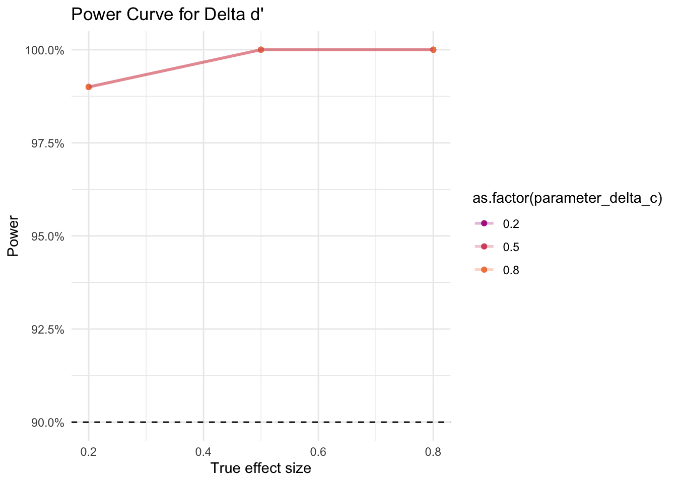

Figure 3: Results of sensitivity analysis for Delta d’. The plot shows the power curve, i.e. the share of statistically significant effects across 100 simulated meta-analyses for each pair of values of d’ (x-axis) and c (color legend).

Code

# plot results
ggplot(plot_data, 
       aes(x = parameter_delta_c, y = power, color = as.factor(parameter_delta_d_prime))) +
  geom_point(size = 1.5, alpha = 0.5) +
  geom_line(size = 1, alpha = 0.3) + 
  # add a horizontal line at 90%, our power_threshold
  geom_hline(aes(yintercept = .9), linetype = 'dashed') + 
  # Prettify!
  theme_minimal() + 
  scale_colour_viridis_d(option = "plasma") + 
  scale_y_continuous(labels = scales::percent) + 
  labs(x = 'True effect size', y = 'Power', 
       title = "Power Curve for Delta c")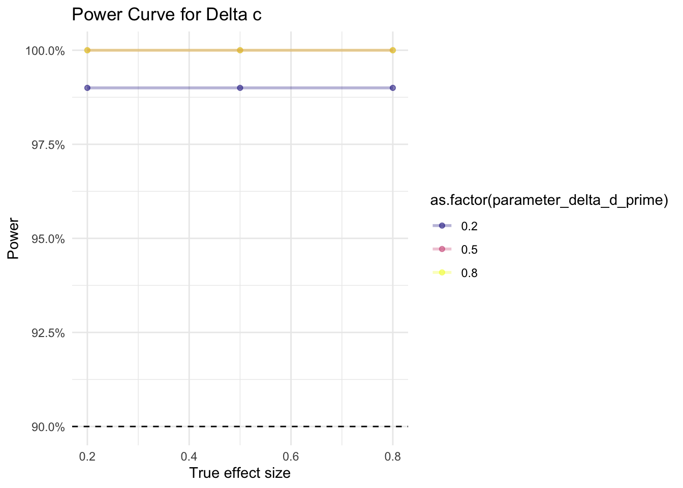

Figure 4: Results of sensitivity analysis for Delta c. The plot shows the power curve, i.e. the share of statistically significant effects across 100 simulated meta-analyses for each pair of values of c (x-axis) and d’ (color legend).

Parameter Recovery

Instead of only checking whether our models find a significant effect or not, we also descriptively check how well our model recovers the data generating parameters across the different samples.

As shown in Figure @ref(fig:sensitivity-parameter-dprime) for d’ and Figure @ref(fig:sensitivity-parameter-c) for c, we find that the distributions of meta-analytic estimates across the 100 samples per pair of effect sizes are centered around the true data generating parameter when the effect size is small (0.2). With an increasing true effect size, however, the estiamte distributions tend to be shifted to the left of the parameter, which suggests that our models consistently underestimate the true effect for larger effect sizes.

Overall, our simulation suggests that (i) given conservative sample size assumptions, we will have large enough statistical power to detect even small effects, and (ii) that our model might slightly underestimate larger true effect sizes, which makes it a conservative estimator.

Code

# custom function for grid labels
custom_labeller <- labeller(
  parameter_delta_c = function(x) paste("Delta c:", x),
  parameter_delta_d_prime = function(x) paste("Delta d':", x)
)

# plot Delta d' estimates
ggplot(sensitivity_data %>% filter(term == "delta d'"), aes(x = estimate)) +
  geom_histogram() +
  geom_vline(aes(xintercept = parameter_delta_d_prime), linetype = "dotted", color = "black") +
  labs(x = "Estimate for Delta d'") + 
  facet_grid(rows = vars(parameter_delta_c), cols = vars(parameter_delta_d_prime), 
    labeller = custom_labeller)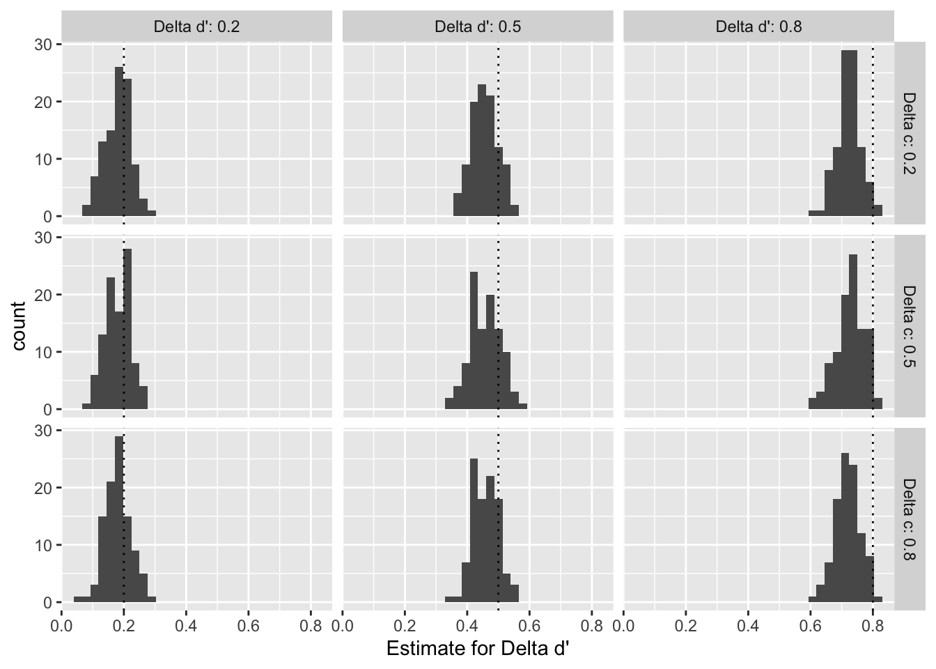

Figure 5: Distributions of Delta d’ across simulated meta-analyses. The plot shows the distribution of meta-analytic estimates, for each combination of Delta d’ and Delta c values.

Code

ggplot(sensitivity_data %>% filter(term == "delta c"), aes(x = estimate)) +
  geom_histogram() +
  geom_vline(aes(xintercept = parameter_delta_c), linetype = "dotted", color = "black") +
  labs(x = "Estimate for Delta c") + 
  facet_grid(cols = vars(parameter_delta_c), rows = vars(parameter_delta_d_prime), 
    labeller = custom_labeller)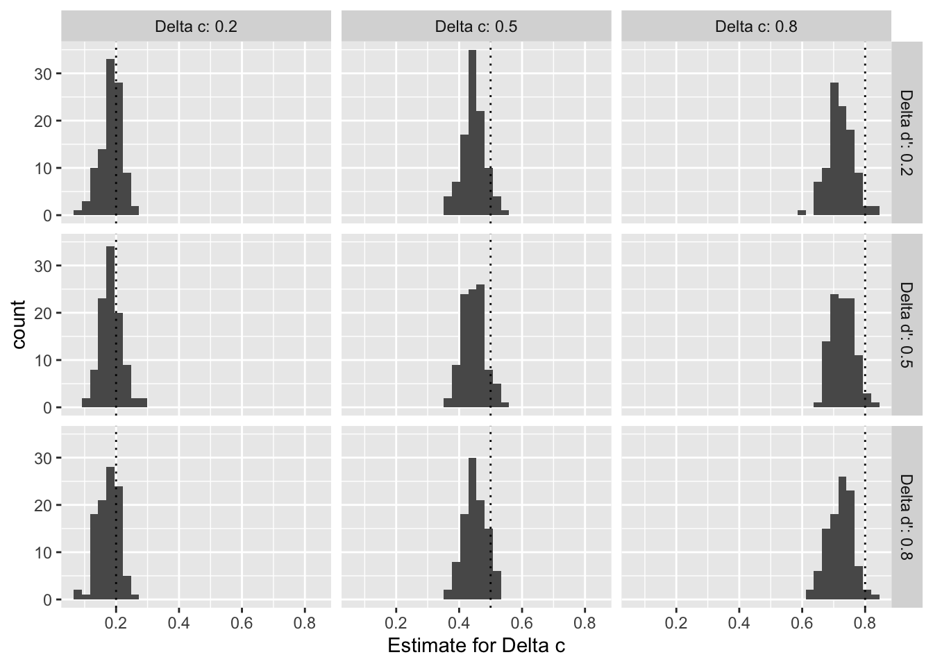

Figure 6: Distributions of Delta c across simulated meta-analyses. The plot shows the distribution of meta-analytic estimates, for each combination of Delta c and Delta d’ values.

Data availability

All simulation data used in this pre-registration is available on the OSF project (https://osf.io/wtxq3/) page or on github (https://github.com/janpfander/meta_interventions_news).

Warning

The project now lives in a new repository: https://github.com/janpfander/meta_misinformation_interventions.

Code availability

All code used to generate this pre-registration and to run the simulations is available on the OSF project (https://osf.io/wtxq3/) page or on github (https://github.com/janpfander/meta_interventions_news).

Warning

The project now lives in a new repository: https://github.com/janpfander/meta_misinformation_interventions.

References

Batailler, Cédric, Skylar M. Brannon, Paul E. Teas, and Bertram Gawronski. 2022. “A Signal Detection Approach to Understanding the Identification of Fake News.” Perspectives on Psychological Science 17 (1): 78–98. https://doi.org/10.1177/1745691620986135.

Batailler, Cédric, Skylar M. Brannon, Paul Teas, and Bertram Gawronski. 2019. “A Signal Detection Approach to Understanding the Identification of Fake News,” September. https://osf.io/uc9me/.

Gawronski, Bertram, Lea S. Nahon, and Nyx L. Ng. 2024. “A Signal-Detection Framework for Misinformation Interventions.” Nature Human Behaviour, October, 1–3. https://doi.org/10.1038/s41562-024-02021-4.

Guay, Brian, Adam J. Berinsky, Gordon Pennycook, and David Rand. 2023. “How to Think about Whether Misinformation Interventions Work.” Nature Human Behaviour 7 (8): 1231–33. https://doi.org/10.1038/s41562-023-01667-w.

Harrer, Mathias, Pim Cuijpers, Furukawa Toshi A, and David D Ebert. 2021. Doing Meta-Analysis with r: A Hands-on Guide. 1st ed. Boca Raton, FL; London: Chapman & Hall/CRC Press.

Higham, Philip A., Ariana Modirrousta-Galian, and Tina Seabrooke. 2024. “Mean Rating Difference Scores Are Poor Measures of Discernment: The Role of Response Criteria.” Current Opinion in Psychology 56 (April): 101785. https://doi.org/10.1016/j.copsyc.2023.101785.

Modirrousta-Galian, Ariana, and Philip A. Higham. 2023. “Gamified Inoculation Interventions Do Not Improve Discrimination Between True and Fake News: Reanalyzing Existing Research with Receiver Operating Characteristic Analysis.” Journal of Experimental Psychology: General.

Pfänder, Jan, and Sacha Altay. 2024. “Spotting False News and Doubting True News: A Meta-Analysis of News Judgments,” February. https://doi.org/10.31219/osf.io/n9h4y.

Appendix

From basic Signal Detection Theory (SDT) to mixed models step-by-step

In this appendix, we explain step-by-step how to go from a by-hand to a generalized linear mixed model (glmm) Signal Detection Theory (SDT) analysis.

Basic Signal Detection Theory

After having classified instances of news ratings according to SDT terminology (Table 5), we can manually calculate SDT outcomes. Table 16 shows by-hand calculated SDT outcomes for the first experiment of our simulated meta-analysis sample.

Code

# Pick a single experiment
data_experiment_1 <- sdt_data %>% 
  filter(unique_experiment_id == "1_1")

# calculate SDT outcomes per condition
sdt_outcomes <- data_experiment_1 %>% 
  group_by(sdt_outcome, condition) %>%
  count() %>% 
  pivot_wider(names_from = sdt_outcome, 
              values_from = n) %>% 
  mutate(
    z_hit_rate = qnorm(hit / (hit + miss)),
    z_false_alarm_rate = qnorm(false_alarm / (false_alarm + correct_rejection)),
    dprime = z_hit_rate - z_false_alarm_rate,
    c = -1 * (z_hit_rate + z_false_alarm_rate) / 2
  ) %>% 
  ungroup()

Code

sdt_outcomes %>% 
  rounded_numbers() %>% 
  kable(
    caption = "SDT outcomes calculated by-hand for Experiment 1 of simulated data.",
    booktabs = TRUE) %>%
  kable_styling(font_size = 8,  # Set a smaller font size
                latex_options = c("scale_down")) # Scale down the table

Table 16: SDT outcomes calculated by-hand for Experiment 1 of simulated data.

condition	correct_rejection	false_alarm	hit	miss	z_hit_rate	z_false_alarm_rate	dprime	c
control	410	90	252	248	0.010	-0.915	0.925	0.453
intervention	407	93	201	299	-0.248	-0.893	0.645	0.570

Our treatment effects are the differences between the control and treatment group. We therefor call them delta_dprime and delta_c here (see Table 17).

Code

treatment_effects <- sdt_outcomes %>%
  select(condition, dprime, c) %>% 
  pivot_wider(
    names_from = condition, 
    values_from = c(dprime, c)
  ) %>% 
  mutate(delta_dprime = dprime_intervention - dprime_control, 
         delta_c = c_intervention - c_control) %>%
  select(starts_with("delta"))

Code

treatment_effects %>% 
  rounded_numbers() %>% 
  kable(
    caption = "SDT treatment effects calculated by-hand for Experiment 1 of simulated data.",
    booktabs = TRUE) %>%
  kable_styling(font_size = 8,  # Set a smaller font size
                latex_options = c("scale_down")) # Scale down the table

Table 17: SDT treatment effects calculated by-hand for Experiment 1 of simulated data.

delta_dprime	delta_c
-0.281	0.118

b. SDT in Generalized Mixed Model (glm)

To obtain test statistics for these outcomes, we can do the equivalent analysis in a generalized linear model (glm), using a probit link function. We use deviation coding for our veracity (fake = -0.5, true = 0.5) and condition (-0.5 = control, 0.5 = intervention) variables. Table 18 shows the results of the glm.

Code

# run model
model_glm <- glm(accuracy ~ veracity_numeric*condition_numeric, data = data_experiment_1, family = binomial(link = "probit"))

# Tidy the model and add the SDT_term column
model_results <- tidy(model_glm, conf.int = TRUE) %>%
  mutate(SDT_term = case_when(
    term == "(Intercept)" ~ "Average c (pooled across all conditions)",
    term == "veracity_numeric" ~ "Average d' (pooled across all conditions)",
    term == "condition_numeric" ~ "Delta c (change in response bias between control and treatment)",
    term == "veracity_numeric:condition_numeric" ~ " Delta d' (change in sensitivity between control and treatment)",
    TRUE ~ "Other"
  ), 
  # reverse c and delta c estimates
  SDT_estimate = ifelse(term == "(Intercept)" | term == "condition_numeric", 
                        -1*estimate, estimate)
  )

Code

# Create a table with kable
model_results %>%
  select(term, estimate, p.value, SDT_estimate, SDT_term) %>%
  kable(
    caption = "Summary of glm results for Experiment 1 of simulated data",
    col.names = c("Term", "Estimate", "p-value", "SDT Estiamte", "SDT Term"),
    digits = 3,
    booktabs = TRUE) %>%
  kable_styling(
    full_width = FALSE, 
    font_size = 10, 
    latex_options = c("scale_down")
  ) %>%
  add_footnote(
    "The model coefficients have the interpretations in terms of SDT as presented here in this table because we use deviation coding for our veracity (fake = -0.5, true = 0.5) and condition (-0.5 = control, 0.5 = intervention) variables.",
    notation = "none"
  )

Table 18: Summary of glm results for Experiment 1 of simulated data

Term	Estimate	p-value	SDT Estiamte	SDT Term
(Intercept)	-0.512	0.000	0.512	Average c (pooled across all conditions)
veracity_numeric	0.785	0.000	0.785	Average d' (pooled across all conditions)
condition_numeric	-0.118	0.053	0.118	Delta c (change in response bias between control and treatment)
veracity_numeric:condition_numeric	-0.281	0.021	-0.281	Delta d' (change in sensitivity between control and treatment)
The model coefficients have the interpretations in terms of SDT as presented here in this table because we use deviation coding for our veracity (fake = -0.5, true = 0.5) and condition (-0.5 = control, 0.5 = intervention) variables.

c. SDT in mixed models

However, this analysis is naive, because it treats all observations (instances of news ratings) as independent. Yet, participants give several ratings, and news ratings from the same participant are not independent of each other.

i. Participant averages

One simple way to account for this dependency is to compute participant-level outcomes, and using these averages as observations. This way, each participant only contributes one data point. Figure @ref(fig:individual-level-plot) shows the distributions of participants’ averages for Experiment 1 of the simulated data. To obtain estimates for our treatment effects \(\Delta c\) and \(\Delta d'\), we can then run a linear regression with condition as a predictor (or do a t-test). The results of these regressions are shown in Table 19.

Code

# calculate SDT outcomes per participant
sdt_participants <- data_experiment_1 %>% 
  drop_na(sdt_outcome) %>% 
  group_by(unique_subject_id, sdt_outcome) %>%
  count() %>%
  ungroup() %>% 
  # Note that currently, not all outcomes appear for participants (e.g. if a participant had only hits and false alarms, correct rejections and misses will not appear). This is a problem later, because when we compute hit and miss rates, the categories that are not appearing will be coded as NA, messing up the calculations. To avoid this, we use the complete() function and ensure that outcomes which do not occur are coded as 0. 
  complete(
    unique_subject_id,
    sdt_outcome, 
    fill = list(n = 0)
  ) %>% 
  # since we want the condition variable in our data, we code it back into there
  left_join(
    sdt_data %>% select(unique_subject_id, condition) %>% distinct()
  ) %>%  
  pivot_wider(names_from = sdt_outcome, 
              values_from = n) %>% 
  # At this point we need to correct for cases when hit rate or false alarm rate take the values of 0 (case in which qnorm(0) = -Inf) or 1 (case in which qnorm(1) = Inf). We follow Batailler in applying log-linear rule correction (Hautus, 1995)
  mutate(
    hit = hit + 0.5,
    miss = miss + 0.5,
    correct_rejection = correct_rejection + 0.5,
    false_alarm = false_alarm + 0.5,
  ) %>% 
  # We can then compute sdt outcomes for each participant
  mutate(
    z_hit_rate = qnorm(hit / (hit + miss)),
    z_false_alarm_rate = qnorm(false_alarm / (false_alarm + correct_rejection)),
    dprime = z_hit_rate - z_false_alarm_rate,
    c = -1 * (z_hit_rate + z_false_alarm_rate) / 2
  ) %>% 
  ungroup()

Code

# plot

# Main plot data: shape data to long format
plot_data <- sdt_participants %>% 
  pivot_longer(c(dprime, c),
               names_to = "outcome", 
               values_to = "value") %>% 
  # make nicer names
  mutate(outcome = ifelse(outcome == "dprime", "D' (sensitivity)", 
                          "C (response bias)"))

# summary data for labels
# table 
summary_data <- plot_data %>% 
  drop_na(value) %>% 
  mutate(valence = ifelse(value > 0, "positive", 
                          ifelse(value == 0, "neutral", 
                                 "negative")
                          )
         ) %>% 
  group_by(valence, outcome) %>% 
  summarize(n_subj = n_distinct(unique_subject_id)) %>% 
    pivot_wider(names_from = outcome, 
              values_from = n_subj) %>% 
  # relative frequency
  ungroup() %>% 
  mutate(
    rel_dprime = `D' (sensitivity)` / sum(`D' (sensitivity)`),
    rel_c =  `C (response bias)` / sum(`C (response bias)`)
    ) %>% 
  pivot_longer(c(rel_dprime, rel_c), 
               names_to = "outcome", 
               values_to = "value") %>% 
  mutate(outcome = ifelse(outcome == "rel_dprime", "D' (sensitivity)", 
                          "C (response bias)"), 
         label = paste0(round(value, digits = 4)*100, " %"),
         x_position = case_when(valence == "negative" ~ -1,
                                valence == "neutral" ~ 0,
                                valence == "positive" ~ 1), 
         y_position = 1.5)

# make plot
individual_level_plot <- ggplot(plot_data, aes(x = value, fill = outcome, color = outcome)) +
  geom_density(alpha = 0.5, adjust = 1.5)+
  # add line at 0
  geom_vline(xintercept = 0, 
             linewidth = 0.5, linetype = "24", color = "grey") +
  # scale
  # scale_x_continuous(breaks = seq(from = -1, to = 1, by = 0.2)) +
  # add labels for share of participants
  geom_label(inherit.aes = FALSE, data = summary_data,
             aes(x = x_position, y = y_position, 
                 label = label),
             alpha = 0.6,
             color = "grey50", size = 3, show.legend = FALSE) +
  # colors 
  scale_color_viridis_d(option = "turbo", begin = 0.25, end = 1)+
  scale_fill_viridis_d(option = "turbo", begin = 0.25, end = 1) +
  # labels and scales
  labs(x = "Z-scores", y = "Density") +
  guides(fill = FALSE, color = FALSE) +
  plot_theme +
  theme(legend.position = "bottom",
        axis.text.y = element_blank(),
        strip.text = element_text(size = 14)) +
  facet_wrap(~outcome)

#individual_level_plot

# Save the plot to a file
ggsave("individual_level_plot.png", individual_level_plot, width = 8, height = 6)

# In the RMarkdown file
knitr::include_graphics("individual_level_plot.png")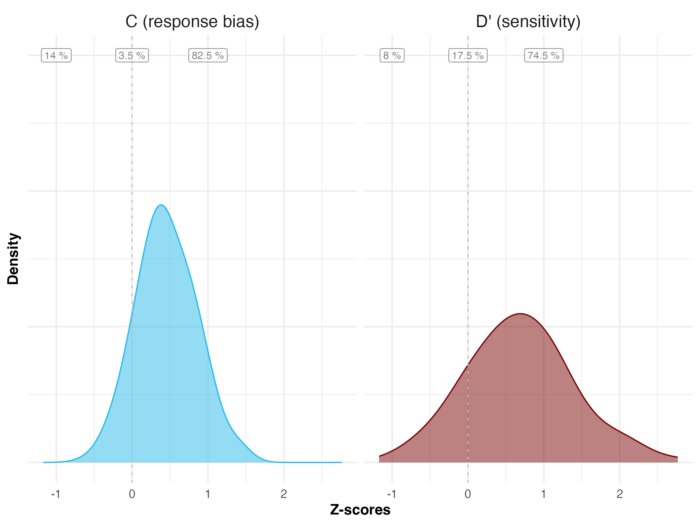

Figure 7: Distribution of participant-level averages for Experiment 1 of the simulated data. The percentage labels (from left to right) represent the share of participants with a negative score, a score of exactly 0, and a positive score, for both measures respectively. Note that when calculating by-participant averages, we follow Batailler et al. (2022) in applying log-linear rule correction. This is particularly relevant for cases when the hit rate or the false alarm rate take the values of 0 (case in which qnorm(0) = -Inf) or 1 (case in which qnorm(1) = Inf).

Code

model_dprime <- lm(dprime ~ condition, data = sdt_participants)
model_c <- lm(c ~ condition, data = sdt_participants)

modelsummary::modelsummary(list("d'" = model_dprime, 
                                "c" = model_c
                                ), 
                           stars = TRUE,
                           output = "kableExtra",
                           title = "SDT outcomes based on a regression on participant-level averages",
                           coef_rename = c("conditionintervention" = "Treatment Effect"),
                           )

Table 19: SDT outcomes based on a regression on participant-level averages

	d'	c
(Intercept)	0.814***	0.402***
	(0.068)	(0.038)
Treatment Effect	−0.263**	0.101+
	(0.096)	(0.054)
Num.Obs.	200	200
R2	0.036	0.017
R2 Adj.	0.031	0.012
AIC	417.5	186.1
BIC	427.4	196.0
Log.Lik.	−205.768	−90.061
RMSE	0.68	0.38
+ p < 0.1, * p < 0.05, p < 0.01, * p < 0.001

By comparing the results of the regression based on participant-level averages (Table 19), to the results of the glm at the rating-level and which glosses over participant dependencies (Table 18), we can see that the estimates for our outcomes \(\Delta c\) and \(\Delta d'\) are slightly different. However, we can account even better for our data structure, and estimate both within and between participant variation separately by using a generalized linear mixed model (glmm).

ii. Mixed model SDT

Using a glm with probit link function as above, we can additionally specify random effects. The result is a generalized linear mixed model (glmm). Adding random effects for participants allows us to model the dependency of data points from the same participant, thereby account for these difference, while not loosing data points as in the participant-averages approach discussed above.

Table 20 shows that, for our simulated experiment 1, the estimates of the glmm are close to, but slightly different from, the initial gml without random effects (Table 18).

Code

# Sometimes these models take time, so we check that time
time <- system.time({
  mixed_model <- glmer(accuracy ~ veracity_numeric + condition_numeric + 
                         veracity_numeric*condition_numeric +
                         (1 + veracity_numeric | unique_subject_id),
                       data = data_experiment_1, 
                       family = binomial(link = "probit"))
})

#print(paste("Elapsed time: ", round(time[3]/60, digits = 2), " minutes"))

# get a tidy version
mixed_model <- tidy(mixed_model, conf.int = TRUE)

Code

# show results
mixed_model <- mixed_model %>%
  mutate(SDT_term = case_when(
    term == "(Intercept)" ~ "Average c (pooled across all conditions)",
    term == "veracity_numeric" ~ "Average d' (pooled across all conditions)",
    term == "condition_numeric" ~ "Delta c (change in -response bias between control and treatment)",
    term == "veracity_numeric:condition_numeric" ~ " Delta d' (change in sensitivity between control and treatment)",
    TRUE ~ "Other"
  ), 
  # reverse c and delta c estimates
  SDT_estimate = ifelse(term == "(Intercept)" | term == "condition_numeric", 
                        -1*estimate, estimate)
  )

mixed_model %>% 
  select(-starts_with("conf")) %>% 
  rounded_numbers() %>% 
  select(-c(effect, group)) %>% 
  kable(
    caption = "Results of a generalize linear mixed model (glmm)",
    booktabs = TRUE) %>%
  kable_styling(font_size = 8,  # Set a smaller font size
                latex_options = c("scale_down")) # Scale down the table

Table 20: Results of a generalize linear mixed model (glmm)

term	estimate	std.error	statistic	p.value	SDT_term	SDT_estimate
(Intercept)	-0.514	0.032	-16.175	0.000	Average c (pooled across all conditions)	0.514
veracity_numeric	0.786	0.062	12.711	0.000	Average d' (pooled across all conditions)	0.786
condition_numeric	-0.119	0.063	-1.892	0.059	Delta c (change in -response bias between control and treatment)	0.119
veracity_numeric:condition_numeric	-0.285	0.123	-2.312	0.021	Delta d' (change in sensitivity between control and treatment)	-0.285
sd__(Intercept)	0.109	NA	NA	NA	Other	0.109
cor__(Intercept).veracity_numeric	1.000	NA	NA	NA	Other	1.000
sd__veracity_numeric	0.090	NA	NA	NA	Other	0.090

Footnotes

Level 1 being the the participant level, i.e. the sampling variation of the original studies, see Harrer et al. (2021).↩︎
visible only in the .html version↩︎