---
title: "Predicting the effects of behavioral interventions on humans with LLMs"
abstract: |
We test the potential of predicting human behavior in survey experiments with behavioral clones—large language model (LLM) generated artificial agents mimicking human participants. To evaluate this potential, we predict the outcomes of a large-scale field experiment (N = ~22,000) to be conducted in the United States. The experiment will test 20 text-based interventions designed to increase trust in climate scientists, assessing a broad range of secondary, outcomes including self-reported attitudes (e.g., support for funding of climate science) and behavioral measures (e.g., donations to a scientific organization). Before the human study is fielded, we will simulate it with behavioral clones using demographically representative U.S. participant profiles. We will lock the simulated dataset and analysis code. Once human data are available, we will compare clone-based predictions to human results for average treatment effect and subgroup heterogeneity. We will also compare how well the LLMS produce outcome distributions, and whether they overemphasize demographic associations (in other words, whether they stereotype). Our study will provide a large-scale, credible benchmark test of LLMs' potential---and limitations---as tools for simulating human subjects in social science research. All analyses in this preregistration are demonstrated on simulated placeholder data with identical structure to the real datasets; no human outcome data have been observed at the time of registration.
# bibliography: ../references.bib
#csl: https://www.zotero.org/styles/apa
date: "2026-05-04"
format:
html:
code-fold: true
toc: true
toc-depth: 4
pdf:
toc: true
toc-depth: 5
include-before-body:
text: |
\clearpage
colorlinks: true
tbl-colwidths: true
header-includes:
- \usepackage{float}
- \floatplacement{figure}{H}
- \floatplacement{table}{H}
- \usepackage{listings}
- \lstset{breaklines=true, basicstyle=\small\ttfamily}
execute:
echo: true
warning: false
message: false
fig-width: 8
fig-height: 5
fig-dpi: 300
---
```{r}
#| label: setup
#| output: false
# packages
library(tidyverse)
library(sandwich)
library(lmtest)
library(marginaleffects)
library(broom)
library(MetBrewer)
library(patchwork)
library(gt)
library(tinytable)
library(here)

# custom functions
source(here("R/functions/statistics.R"))
source(here("R/functions/plots.R"))
source(here("R/functions/tables.R"))
source(here("R/functions/reporting.R"))

# simulated (random) data
human_data <- readRDS(here("data/simulation_preregistration/human_data_preregistration.rds"))
llm_data   <- readRDS(here("data/simulation_preregistration/llm_data_preregistration.rds"))

# Preregistered random split of human sample into two halves.
# human_data_1 is the reference half used in all primary analyses.
# human_data_2 is the baseline comparator (human-human ceiling for all metrics).
set.seed(42)
split_ids    <- sample(unique(human_data$id), size = floor(length(unique(human_data$id)) / 2))
human_data_1 <- human_data |> filter(id %in% split_ids)
human_data_2 <- human_data |> filter(!id %in% split_ids)

# interventions
interventions <- read_csv(here("data/interventions.csv"))

# actual data later
# human_data  <- readRDS("data/cleaned_llm.rds")
# llm_data <- readRDS("data/cleaned_llm.rds")
```
::: {.callout-important}
**Placeholder data.** Both datasets used throughout are simulated random noise with the correct structure. The analysis code will be applied to real human and LLM clone data without modification once both are available.
:::
## Motivation
The aim of this project is to understand how well large language models (LLMs) can simulate human behavior in survey experiments.
Large language models (LLMs) are trained on extensive human-generated data. Consequently, they reproduce patterns of human judgment and reasoning [@binzUsingCognitivePsychology2023; @aherUsingLargeLanguage2023]. In controlled, text-based interactions, humans sometimes struggle to distinguish between responses generated by LLMs and those produced by other humans [@jonesPeopleCannotDistinguish2025; but see @paganComputationalTuringTest2025].
This apparent capability of LLMs to mimic human behavior has generated substantial interest among social scientists. Running surveys and experiments with human subjects is costly and time-consuming. If LLMs could reliably approximate human behavior, they would offer a fast and low-cost alternative. While it seems unrealistic at this point that LLMs could substitute human subjects entirely [see, e.g., @schroderLargeLanguageModels2025a], they might still open up substantial new opportunities for social science research. Academic publishing systems tend to incentivize positive results [@nosekScientificUtopiaII2012; @smaldinoNaturalSelectionBad2016], which can discourage the testing of novel or high-risk ideas. Approximative LLM simulations could serve as a low-risk tool for pretesting such novel ideas before committing resources to human data collection. LLMs could also help testing the boundaries of established theories. Scientific theories---at least in the social sciences---are often highly context-dependent. To improve theory building, researchers have called for more systematic exploration of these contextual variations [@almaatouqPlaying20Questions2022a]. LLMs could make such exploration more feasible: they could simulate a multitude of variations of an experiment, thereby pointing researchers to critical context factors that could be tested in follow-up studies on human participants.
Recent studies have demonstrated promising results for LLMs in simulating public opinion [@kaiserSimulatingHumanOpinions2025; @wangLargeLanguageModels2025; @argyleOutOneMany2023; @durmusMeasuringRepresentationSubjective2024; @santurkarWhoseOpinionsLanguage2023; @bisbeeSyntheticReplacementsHuman2024; @shresthaWEIRDCanSynthetic2024] and in predicting the outcomes of experiments with human participants [@hewittPredictingResultsSocial2025; @chenPredictingFieldExperiments2025; @huSimBenchBenchmarkingAbility2025; @guoEstimatingCausalEffects2025; @lippertCanLargeLanguage2024; @bisbeeSyntheticReplacementsHuman2024]. At the same time, other work has identified important limitations of LLM simulations, including systematic misrepresentation of certain identity groups [@wangLargeLanguageModels2025], a general tendency of overestimating experimental effects [@doudkinAIPersuadingAI2025; @cuiCanAIReplace2024], and high volatility of simulation results, depending on model and prompt choice [@schroderLargeLanguageModels2025a].
Currently, interpreting these mixed findings is difficult, as most existing studies face at least one of the following limitations. First, some studies rely on already published experiments, raising concerns that LLMs may have been trained on the very data they are asked to simulate. These studies might only test LLMs capacity to reproduce, but not to predict. Second, even studies that plausibly rely on unpublished data are rarely preregistered. Given that LLM performance is highly sensitive to model choice and prompting, preregistered predictions are crucial for credible evaluation. Third, some studies operate at the experiment level, providing LLMs with a full description of the study and requesting a single aggregate prediction. While informative about average effects, this approach precludes the analysis of individual-level heterogeneity.
In this project, we aim to provide a robust test of how well LLMs can simulate human behavior in survey experiments. We address limitations of previous studies by leveraging a unique opportunity to evaluate LLM simulations in the context of a large-scale field experiment, involving approximately 21,000 participants from the United States (US), testing 20 text-based interventions designed to increase trust in climate scientists. The study assesses a broad range of outcomes, including self-reported attitudes (e.g., trust in scientists) and behavioral measures (e.g., donations to a scientific organization). Before running the study with human participants, we will use multiple LLMs and prompting strategies to simulate individual-level survey responses representative of the US population. We will then collect the human data and test how closely they match the data simulated by the LLMs. This design allows for a large-scale, credible benchmark test of LLMs' potential---and limitations---as tools for simulating human subjects in social science research.
## Research Questions
The main outcome of the megastudy is trust in climate scientists, but several secondary and tertiary outcomes are preregistered. Analyses are organized in three sections that mirror one another: we first examine average effects, then subgroup differences, and finally demographic calibration at the individual level.
**Section 1 — Average Treatment Effects.** We ask (a) how well LLM clones predict the average treatment effect (ATE) of each intervention across all outcomes, and (b) to which extent clones produce similar response distributions for the different outcomes (in the control condition).
**Section 2 — Subgroup Effects.** We ask (a) how closely clones predict differences in intervention effects across six demographic moderators (gender, age, race, education, income, partisan identity) for all outcomes, and (b) how closely within-subgroup response distributions in the control condition match between humans and clones for the primary outcome.
**Section 3 — Demographic Baseline Calibration.** Independent of treatment effects, we ask whether clone baseline outcome levels are calibrated to the assigned demographic profile: (a) do clones reproduce the correct group mean for each demographic group in the control condition, and (b) do demographic variables predict clone outcomes with the same magnitude as in humans, or do clones over-rely on demographic cues? Analyses are run separately for all outcomes; results are illustrated with the primary outcome (`trust_multidimensional`).
## Data
### Human data
The human dataset will come from a large-scale between-subjects field experiment to be conducted in the United States (N ≈ 22,000). Participants will be randomly assigned to one of 20 text-based interventions designed to increase trust in climate scientists, or to a control condition. The human study is preregistered separately ([https://doi.org/10.5281/zenodo.20160212](https://doi.org/10.5281/zenodo.20160212)). **No human data has been colleced at the moment of registering this study.**
To provide a reference baseline for interpreting LLM performance, we split the human sample into two equal halves using a preregistered random split (`set.seed(42)`). **Human 1** (the reference half) is used in all primary analyses and serves as the ground-truth against which both LLMs and the second human half are compared. **Human 2** provides a human-human reference: the similarity between the two halves quantifies how well human data predict other human data, which is the upper bound for any predictive method. All comparison tables and the pooled scatter plot report metrics for both comparisons side by side.
#### Interventions
@tbl-interventions provides a summary of the different interventions tested in the megastudy. In this project, we only generate LLM clone responses for non-interactive interventions. As a result, we only test 16 interventions (none of the three LLM-chatbot interventions, neither the 'Value similarity' quiz intervention).
```{r}
#| label: build-tbl-interventions
# build table data with category headers manually

intervention_table_data <- interventions |>
  select(title, summary, tag) |>
  mutate(
    tag = factor(tag, levels = c(
      "Collaboration and peer-review",
      "Scientific methods and results",
      "Applications and impact",
      "Others' endorsement",
      "Values",
      "LLM-chatbot",
      "Other"
    ))
  ) |>
  arrange(tag) |>
  mutate(number = as.character(row_number())) |>
  group_by(tag) |>
  group_modify(~ bind_rows(
    tibble(title = as.character(.y$tag), summary = ""),
    .x
  )) |>
  ungroup() |>
  mutate(` ` = ifelse(title %in% levels(tag), "", number)) |>
  select(` `, title, summary) |>
  rename(`Intervention Title` = title,
         Summary = summary)

# identify header rows
header_rows <- which(intervention_table_data$` ` == "")

intervention_table <- intervention_table_data |>
  tt(width = c(0.05, 0.25, 0.70)) |>
  format_tt(escape = TRUE) |>
  style_tt(align = "l", alignv = "t") |>
  style_tt(i = 0, bold = TRUE) |>
  style_tt(i = header_rows, bold = TRUE, j = 2, colspan = 2) |>
  style_tt(fontsize = 0.85)
```
```{r}
#| label: tbl-interventions
#| tbl-cap: "Overview of interventions included in the megastudy."
#| eval: !expr "!knitr::is_latex_output()"
intervention_table
```
```{r}
#| eval: !expr "knitr::is_latex_output()"
intervention_table |>
  theme_latex(multipage = TRUE, rowhead = 1,
              outer = "caption={Overview of interventions included in the megastudy.}, label={tbl-interventions}")
```
#### Outcomes
Outcomes are organized in three tiers reflecting theoretical proximity to the primary target of the interventions:
- **Primary**: `trust_multidimensional` — a composite measure of trust in climate scientists averaging four subdimensions (competence, integrity, benevolence, openness), each assessed with three items (12 items total, scored 0–100). This is the pre-specified main endpoint.
- **Secondary** (five outcomes): single-item trust (`trust_post`), single-item distrust (`distrust_post`), perceptions of science funding (`funding_perceptions`), perceived appropriate policy role of scientists (`policy_role_mean`), and institutional trust (`inst_trust_mean`).
- **Tertiary** (five outcomes): climate belief (`belief_post`), climate concern (`concern_mean`), general climate policy support (`policy_general`), specific climate policy support (`policy_specific_mean`), and pro-climate behavior intentions (`behavior_mean`).
- **Binary**: newsletter sign-up (`newsletter_signup`) — a behavioral outcome recording whether the participant subscribed to a climate science newsletter. Analyzed separately with logistic regression; excluded from distribution analyses.
ATE analyses cover all 13 outcomes. Analyses that break results down by outcome — response distribution comparisons (Section 1) and subgroup heterogeneity (Section 2) — use an illustrative subset of four outcomes spanning the tiers: multidimensional trust (primary), donation to AMS (secondary), funding perceptions (secondary), and general climate policy support (tertiary). Subgroup analyses use six demographic moderators: gender, age band, race, education, income, and partisan identity.
### LLM generated data
#### Profiles
Clone profiles were constructed by drawing 9,000 individuals from four recent waves of the General Social Survey (GSS; 2018, 2021, 2022, 2024). Within-year normalized sampling weights were applied so that each wave contributes equal sampling probability to the pool, while preserving within-year relative weights. Each profile was assigned to exactly one experimental condition (between-subjects, matching the human study design). The exact procedure is documented in the project repository.
Profiles encode the following demographic characteristics: age, sex, race/ethnicity (racial self-identification and Hispanic origin), educational attainment, household income, household size, self-identified social class, U.S. region, partisan identification, political ideology, religious affiliation, religious intensity, and confidence in the scientific community. Each clone then completed the survey experiment under the same conditions as human participants.
```{r}
#| label: tbl-profile-completeness
#| tbl-cap: "Missing values per variable by GSS wave. Column headers show the wave year and total N for that wave in brackets."
profiles <- read_csv(here("clone_profiles", "profiles.csv"), show_col_types = FALSE)

meta_vars <- c("profile_id", "year", "id", "wtssps", "w_pooled",
               "profile_basic", "profile_detailed")
prof_vars <- setdiff(names(profiles), meta_vars)
yrs       <- sort(unique(profiles$year))

yr_ns <- profiles |> count(year) |> deframe()

comp_tbl <- prof_vars |>
  map_dfr(\(v) {
    row <- tibble(Variable = v)
    for (yr in yrs) {
      d <- profiles |> filter(year == yr) |> pull(all_of(v))
      row[[paste0(yr, " (N=", yr_ns[[as.character(yr)]], ")")]] <- sum(is.na(d))
    }
    row
  })

comp_tbl |>
  tt() |>
  style_tt(j = 1, align = "l") |>
  style_tt(j = seq(2, ncol(comp_tbl)), align = "r") |>
  style_tt(i = 0, bold = TRUE)
```
```{r}
#| label: tbl-profile-demographics
#| tbl-cap: "Distribution of key quota variables in the LLM clone profile pool (N = 9,000)."
race_var <- if ("racecen1" %in% names(profiles)) "racecen1" else "race"

age_tbl <- profiles |>
  mutate(Category = cut(age,
    breaks = c(17, 29, 44, 59, Inf),
    labels = c("18–29", "30–44", "45–59", "60+")
  )) |>
  count(Category) |>
  mutate(pct = round(100 * n / sum(n), 1), group = "Age")

sex_tbl <- profiles |>
  count(Category = sex) |>
  mutate(pct = round(100 * n / sum(n), 1), group = "Sex")

race_tbl <- profiles |>
  count(Category = .data[[race_var]]) |>
  mutate(pct = round(100 * n / sum(n), 1), group = "Race / Ethnicity")

demo_tbl <- bind_rows(age_tbl, sex_tbl, race_tbl) |>
  mutate(Category = as.character(Category))

demo_tbl |>
  select(Category, n, pct) |>
  rename(N = n, "%" = pct) |>
  tt(width = 0.5) |>
  group_tt(i = list(
    "Age"              = which(demo_tbl$group == "Age")[1],
    "Sex"              = which(demo_tbl$group == "Sex")[1],
    "Race / Ethnicity" = which(demo_tbl$group == "Race / Ethnicity")[1]
  )) |>
  style_tt(align = "l") |>
  style_tt(i = 0, bold = TRUE) |>
  style_tt(i = "groupi", bold = TRUE) |>
  format_tt(escape = TRUE)
```
#### Prompt
::: {.content-visible when-format="html"}
<pre style="white-space: pre-wrap;">"You are an expert in simulating participants in behavioral and social science studies. You will be given a detailed profile of a specific U.S. resident and asked to respond to survey questions exactly as that person would.\n\n### Participant Profile\n- Age: [AGE] (current year: 2026)\n- Sex: [SEX]\n- Race: [RACECEN1]\n- Highest educational degree: [DEGREE]\n- Household income (GSS bracket): [INCOME16]\n- Household size: [HOMPOP]\n- Self-described social class: [CLASS]\n- Census region: [REGION]\n- Living area: [SRCBELT]\n- Party identification: [PARTYID]\n- Political views (liberal-conservative): [POLVIEWS]\n- Religion: [RELIG]\n- Strength of religious affiliation: [RELITEN]\n- Identify as a born-again or Evangelical Christian: [REBORN]\n- Trust in the scientific community: [CONSCI]\n\nGive the answer this specific person would actually give, even if it is blunt, contradictory, or reflects limited information."</pre>
:::
::: {.content-visible when-format="pdf"}
```{=latex}
\begin{lstlisting}
"You are an expert in simulating participants in behavioral and social science studies. You will be given a detailed profile of a specific U.S. resident and asked to respond to survey questions exactly as that person would.\n\n### Participant Profile\n- Age: [AGE] (current year: 2026)\n- Sex: [SEX]\n- Race: [RACECEN1]\n- Highest educational degree: [DEGREE]\n- Household income (GSS bracket): [INCOME16]\n- Household size: [HOMPOP]\n- Self-described social class: [CLASS]\n- Census region: [REGION]\n- Living area: [SRCBELT]\n- Party identification: [PARTYID]\n- Political views (liberal-conservative): [POLVIEWS]\n- Religion: [RELIG]\n- Strength of religious affiliation: [RELITEN]\n- Identify as a born-again or Evangelical Christian: [REBORN]\n- Trust in the scientific community: [CONSCI]\n\nGive the answer this specific person would actually give, even if it is blunt, contradictory, or reflects limited information."
\end{lstlisting}
```
:::
#### Simulation
The simulation uses the Qualtrics file of the human study to walk the each LLM through the study as a participant would experience it, with minor deviations. For details, see [github.com/yarakyrychenko/llm-participants](github.com/yarakyrychenko/llm-participants).
#### Data
This preregistration demonstrates the full analysis workflow using data from a single model. At the time of preregistration, complete simulations exist for two models: OpenAI GPT-4o mini and Google Gemini 2.5 Flash Lite. The data for these two models is registered on Zenodo before data collection ([https://doi.org/10.5281/zenodo.20167059](https://doi.org/10.5281/zenodo.20167059)).
Due to API request limitations, simulation data from other models are not available at the point of registration. These simulations need to be be conducted in smaller batches. However, the code for running these simulations is preregistered. For a time-stamped release of the code, see [https://github.com/yarakyrychenko/llm-participants/releases/tag/v1.0.0](https://github.com/yarakyrychenko/llm-participants/releases/tag/v1.0.0).
## Measures
```{r}
#| label: variables
outcomes_primary <- "trust_multidimensional"

outcomes_secondary <- c(
  "trust_post", "distrust_post",
  #"donation_ams",
  "funding_perceptions", "policy_role_mean", "inst_trust_mean"
)

outcomes_binary <- "newsletter_signup"

outcomes_tertiary <- c(
  "belief_post", "concern_mean", "policy_general",
  "policy_specific_mean", "behavior_mean"
)

outcomes_continuous <- c(outcomes_primary, outcomes_secondary, outcomes_tertiary)

# Illustrative subset for by-outcome breakdowns (distributions, moderator detail)
outcomes_illustrative <- c(
  "trust_multidimensional",
  "donation_ams",
  "funding_perceptions",
  "policy_general"
)

trust_dimensions <- c(
  "trust_competence", "trust_integrity", "trust_benevolence", "trust_openness"
)

trust_items <- c(
  paste0("trust_competence_",  1:3),
  paste0("trust_integrity_",   1:3),
  paste0("trust_benevolence_", 1:3),
  paste0("trust_openness_",    1:3)
)

moderators_cat <- c("gender", "age_band", "race", "education", "income", "party")

outcome_label_map <- c(
  trust_multidimensional = "Multidimensional trust (primary)",
  trust_post             = "Overall trust",
  distrust_post          = "Distrust",
  donation_ams           = "Donation to AMS ($)",
  newsletter_signup      = "Newsletter sign-up",
  funding_perceptions    = "Funding perceptions",
  policy_role_mean       = "Policy role",
  inst_trust_mean        = "Institutional trust",
  belief_post            = "Climate belief",
  concern_mean           = "Climate concern",
  policy_general         = "General climate policy",
  policy_specific_mean   = "Specific climate policy",
  behavior_mean          = "Pro-climate behavior"
)
```
::: {.callout-note}
**Illustrative outcomes.** Analyses that break down results by outcome — response distributions (Section 1) and subgroup heterogeneity (Section 2) — report results for an illustrative subset of four outcomes spanning the primary, secondary, and tertiary tiers: multidimensional trust (primary), donation to AMS, funding perceptions, and general climate policy. The preregistered ATE comparison (Section 1, ATE Recovery) covers all outcomes.
:::
## Comparison Functions
Two helper functions operationalize the comparison metrics. They are applied symmetrically to human and LLM clone model outputs throughout the document.
### Comparison metrics
`compare_estimates()` is used throughout — for ATEs (RQ1), moderator interaction estimates (RQ3), and secondary analyses. It computes six metrics, reported in increasing order of strictness. The rationale for this ordering is to locate precisely *where* clone performance breaks down: a clone dataset might pass the weakest test (getting directions right) while failing a stricter one (magnitude equivalence), and knowing at which rung the ladder breaks is more informative than any single pass/fail verdict.
- **Directional agreement (%)** — *least strict.* % of estimates with the same sign as the human estimate. Chance performance is 50%. Answers: do clones at least identify the direction of each effect?
- **Spearman ρ** — rank correlation of point estimates. Answers: do clones rank interventions in the same order as humans? Insensitive to scale or offset; a clone that inflates all effects equally would still score ρ = 1.
- **Pearson r** — linear correlation of point estimates. Captures proportionality between clone and human estimates but not absolute level.
- **Inferential agreement (%)** — % of estimates with the same BH-adjusted conclusion (significantly positive, significantly negative, or non-significant at α = .05). Requires getting both magnitude and uncertainty right; answers whether a researcher using clones would reach the same inferential decision as one using human data.
- **RMSE** — root mean squared error in outcome units. Captures average absolute magnitude error; scale-dependent and therefore not comparable across outcomes.
- **TOST (%)** — *most strict.* % of individual estimate pairs passing an equivalence test with bound Δ_k = 0.5 × |ATE_human_k|. Equivalence is declared (two one-sided tests, α = .05) when the clone estimate falls within ±50% of the human estimate. Note: near-zero human ATEs shrink Δ_k proportionally, making equivalence harder to achieve.
```{r, results='asis'}
#| label: fn-compare-estimates
print_a_function_from_file("compare_estimates")
```
### Distribution comparison metrics
`compare_distributions()` compares response distributions for a single condition and outcome using three metrics, again in increasing order of strictness:
- **Variance ratio** (clone / human variance) — *least strict.* Captures only one aspect of distributional similarity — relative spread. A ratio of 1 means equal dispersion; does not assess shape.
- **OVL (overlapping coefficient)** — proportion of the total area shared between the two kernel density estimates; 1 = identical distributions, 0 = no overlap. Summarises overall shape similarity.
- **KS D-statistic** — *most strict.* Maximum absolute gap between the two empirical CDFs at any point on the response scale; 0 = indistinguishable CDFs everywhere. Sensitive to local departures that OVL might average away.
```{r, results='asis'}
#| label: fn-compare-distributions
print_a_function_from_file("compute_ovl")
```
### Calibration regression
Correlation between human and clone ATEs tells us only whether the two effect-size vectors *covary* — whether interventions that produce large effects in humans also produce large effects in clones. However, correlation does not capture baseline differences or multiplicative scaling: clones could underestimate the control-condition baseline and inflate every effect by a factor of two while still yielding Pearson r = 1. Calibration regression separates these two failure modes — additive bias and proportionality.
`run_calibration()` regresses human ATEs on LLM clone ATEs: `ATE_human = α + β × ATE_clone`. The intercept α captures additive bias: α > 0 means clones systematically underestimate human ATEs (an offset must be added to recover them), α < 0 means they overestimate. The slope β captures proportionality: β = 1 is perfect scaling (clone effects move 1:1 with human effects), β > 1 means clone effects are compressed relative to humans (too small in absolute magnitude), β < 1 means they are exaggerated. We report 95% confidence intervals for both parameters and R² as the share of human-ATE variance linearly recoverable from clone ATEs.
We then test calibration at two levels of strictness. The **joint F-test of (α = 0, β = 1)** is the omnibus test of perfect calibration: it asks whether clone ATEs can be read directly as estimates of human ATEs, with no correction at all. A significant result means the null of perfect calibration is rejected — clone ATEs are not a direct substitute for human ATEs. The **slope-only F-test of (β = 1)** asks the weaker diagnostical question whether clone effects are *proportionally* calibrated, i.e. whether a one-unit difference in a clone ATE corresponds to a one-unit difference in a human ATE, while permitting a constant additive offset α. This additional test is meaningful because proportional calibration is the more practically relevant criterion: in real-world applications, additive bias is relatively easy to correct with a single human anchor condition, whereas a slope distortion reflects a deeper failure in how clones translate to humans and cannot be removed without re-estimating β.
```{r, results='asis'}
#| label: fn-calibration
print_a_function_from_file("run_calibration")
```
### Demographic baseline and predictability metrics
`compare_demographic_baselines()` computes, for each moderator, the Pearson correlation and RMSE between human and clone cell means in the control condition. `compare_demographic_predictability()` fits separate OLS regressions of the outcome on each moderator plus condition fixed effects, returning R² and dummy-coded coefficients for humans and clones.
```{r, results='asis'}
#| label: fn-demographic-baselines
print_a_function_from_file("compare_demographic_baselines")
```
```{r, results='asis'}
#| label: fn-demographic-predictability
print_a_function_from_file("compare_demographic_predictability")
```
## 1. Average Treatment Effects
### ATE Recovery
For each intervention, the average treatment effect (ATE) is the difference in mean outcome between participants assigned to that intervention and those in the control condition. We estimate ATEs by running `run_main_treatment_model()` — OLS with HC2 heteroskedasticity-robust standard errors and BH-adjusted p-values — on human and LLM clone data separately for each preregistered outcome. For `newsletter_signup` (binary), we use `run_main_treatment_model_binary()`, which returns marginal effects on the probability scale.
We report the six comparison metrics in increasing order of strictness, from directional agreement (do clones identify the correct direction of each effect?) to TOST equivalence testing (does each clone ATE fall within a preregistered tolerance of the corresponding human ATE?). We first report metrics pooled across all outcomes — `r (length(outcomes_continuous) + length(outcomes_binary)) * 20` estimate pairs in total — to maximize statistical power, then break down by outcome and zoom in on the primary outcome. All models are fit first.
```{r}
#| label: rq1-all
# Run and store all models (avoids re-fitting in later chunks)
ate_model_results <- map(outcomes_continuous, function(out) {
  list(
    h  = run_main_treatment_model(human_data_1, outcome = out),
    l  = run_main_treatment_model(llm_data,     outcome = out),
    h2 = run_main_treatment_model(human_data_2, outcome = out)
  )
}) |> set_names(outcomes_continuous)

# Binary outcome: marginal effects on probability scale
h_bin  <- run_main_treatment_model_binary(human_data_1, "newsletter_signup")
l_bin  <- run_main_treatment_model_binary(llm_data,     "newsletter_signup")
h2_bin <- run_main_treatment_model_binary(human_data_2, "newsletter_signup")

# References to primary outcome models for the primary subsection below
h_primary  <- ate_model_results[["trust_multidimensional"]]$h
l_primary  <- ate_model_results[["trust_multidimensional"]]$l
h2_primary <- ate_model_results[["trust_multidimensional"]]$h2

# Extract ATE pairs with SE and adjusted p-value from a model result tibble
prep_ate <- function(df) {
  df |>
    select(condition, estimate) |>
    mutate(
      se    = if ("std.error"        %in% names(df)) df$std.error        else NA_real_,
      p_adj = if ("p.value_adjusted" %in% names(df)) df$p.value_adjusted else NA_real_
    )
}

# Pool ATE pairs across all outcomes (continuous + binary)
pooled_ates <- bind_rows(
  map_dfr(outcomes_continuous, function(out) {
    inner_join(
      prep_ate(ate_model_results[[out]]$h) |>
        rename(estimate_h = estimate, se_h = se, p_adj_h = p_adj),
      prep_ate(ate_model_results[[out]]$l) |>
        rename(estimate_l = estimate, se_l = se, p_adj_l = p_adj),
      by = "condition"
    ) |> mutate(outcome = out)
  }),
  inner_join(
    prep_ate(h_bin$marginal_effects) |>
      rename(estimate_h = estimate, se_h = se, p_adj_h = p_adj),
    prep_ate(l_bin$marginal_effects) |>
      rename(estimate_l = estimate, se_l = se, p_adj_l = p_adj),
    by = "condition"
  ) |> mutate(outcome = "newsletter_signup")
) |>
  mutate(
    tier = case_when(
      outcome == outcomes_primary                          ~ "Primary",
      outcome %in% c(outcomes_secondary, outcomes_binary) ~ "Secondary",
      TRUE                                                ~ "Tertiary"
    ),
    outcome_label = outcome_label_map[outcome]
  )

# Human 1 vs. Human 2 ATE pairs (same structure as pooled_ates)
pooled_ates_h2 <- bind_rows(
  map_dfr(outcomes_continuous, function(out) {
    inner_join(
      prep_ate(ate_model_results[[out]]$h) |>
        rename(estimate_h = estimate, se_h = se, p_adj_h = p_adj),
      prep_ate(ate_model_results[[out]]$h2) |>
        rename(estimate_h2 = estimate, se_h2 = se, p_adj_h2 = p_adj),
      by = "condition"
    ) |> mutate(outcome = out)
  }),
  inner_join(
    prep_ate(h_bin$marginal_effects) |>
      rename(estimate_h = estimate, se_h = se, p_adj_h = p_adj),
    prep_ate(h2_bin$marginal_effects) |>
      rename(estimate_h2 = estimate, se_h2 = se, p_adj_h2 = p_adj),
    by = "condition"
  ) |> mutate(outcome = "newsletter_signup")
) |>
  mutate(
    tier = case_when(
      outcome == outcomes_primary                          ~ "Primary",
      outcome %in% c(outcomes_secondary, outcomes_binary) ~ "Secondary",
      TRUE                                                ~ "Tertiary"
    ),
    outcome_label = outcome_label_map[outcome]
  )

# Per-outcome summary metrics
ate_metrics <- map_dfr(outcomes_continuous, function(out) {
  compare_estimates(ate_model_results[[out]]$h, ate_model_results[[out]]$l) |>
    mutate(outcome = out)
})

calib_metrics <- map_dfr(outcomes_continuous, function(out) {
  run_calibration(ate_model_results[[out]]$h, ate_model_results[[out]]$l) |>
    mutate(outcome = out)
})

ate_metrics <- bind_rows(
  ate_metrics,
  compare_estimates(h_bin$marginal_effects, l_bin$marginal_effects) |>
    mutate(outcome = "newsletter_signup")
) |>
  mutate(
    tier = case_when(
      outcome == outcomes_primary                          ~ "Primary",
      outcome %in% c(outcomes_secondary, outcomes_binary) ~ "Secondary",
      TRUE                                                ~ "Tertiary"
    ),
    outcome_label = outcome_label_map[outcome]
  )

calib_metrics <- bind_rows(
  calib_metrics,
  run_calibration(h_bin$marginal_effects, l_bin$marginal_effects) |>
    mutate(outcome = "newsletter_signup")
) |>
  mutate(
    tier = case_when(
      outcome == outcomes_primary                          ~ "Primary",
      outcome %in% c(outcomes_secondary, outcomes_binary) ~ "Secondary",
      TRUE                                                ~ "Tertiary"
    ),
    outcome_label = outcome_label_map[outcome]
  )

# Calibration regression for Human 1 vs. Human 2 (baseline ceiling)
calib_metrics_h2 <- map_dfr(outcomes_continuous, function(out) {
  run_calibration(ate_model_results[[out]]$h, ate_model_results[[out]]$h2) |>
    mutate(outcome = out)
})

calib_metrics_h2 <- bind_rows(
  calib_metrics_h2,
  run_calibration(h_bin$marginal_effects, h2_bin$marginal_effects) |>
    mutate(outcome = "newsletter_signup")
) |>
  mutate(
    tier = case_when(
      outcome == outcomes_primary                          ~ "Primary",
      outcome %in% c(outcomes_secondary, outcomes_binary) ~ "Secondary",
      TRUE                                                ~ "Tertiary"
    ),
    outcome_label = outcome_label_map[outcome]
  )

# Pooled summary row — prepended to ate_metrics so it appears at the top of tbl-rq1
pooled_row <- pooled_ates |>
  mutate(
    delta      = 0.5 * abs(estimate_h),
    diff       = estimate_h - estimate_l,
    se_diff    = sqrt(se_h^2 + se_l^2),
    p_lower    = pnorm((diff + delta) / se_diff, lower.tail = FALSE),
    p_upper    = pnorm((diff - delta) / se_diff),
    p_tost     = pmax(p_lower, p_upper),
    equivalent = p_tost < 0.05,
    same_sign  = sign(estimate_h) == sign(estimate_l),
    infer_h    = case_when(
      !is.na(p_adj_h) & p_adj_h < 0.05 & estimate_h > 0 ~ "sig_positive",
      !is.na(p_adj_h) & p_adj_h < 0.05 & estimate_h < 0 ~ "sig_negative",
      TRUE ~ "not_significant"
    ),
    infer_l    = case_when(
      !is.na(p_adj_l) & p_adj_l < 0.05 & estimate_l > 0 ~ "sig_positive",
      !is.na(p_adj_l) & p_adj_l < 0.05 & estimate_l < 0 ~ "sig_negative",
      TRUE ~ "not_significant"
    )
  ) |>
  summarise(
    spearman_rho    = cor(estimate_h, estimate_l, method = "spearman",
                          use = "pairwise.complete.obs"),
    pearson_r       = cor(estimate_h, estimate_l, use = "pairwise.complete.obs"),
    rmse            = NA_real_,
    directional_pct = mean(same_sign,  na.rm = TRUE) * 100,
    inferential_pct = mean(infer_h == infer_l, na.rm = TRUE) * 100,
    tost_pct        = mean(equivalent, na.rm = TRUE) * 100
  ) |>
  mutate(outcome = "pooled", tier = "All outcomes", outcome_label = "All outcomes")

# Per-outcome summary metrics for Human 1 vs. Human 2 (baseline ceiling)
ate_metrics_h2 <- map_dfr(outcomes_continuous, function(out) {
  compare_estimates(ate_model_results[[out]]$h, ate_model_results[[out]]$h2) |>
    mutate(outcome = out)
})

ate_metrics_h2 <- bind_rows(
  ate_metrics_h2,
  compare_estimates(h_bin$marginal_effects, h2_bin$marginal_effects) |>
    mutate(outcome = "newsletter_signup")
) |>
  mutate(
    tier = case_when(
      outcome == outcomes_primary                          ~ "Primary",
      outcome %in% c(outcomes_secondary, outcomes_binary) ~ "Secondary",
      TRUE                                                ~ "Tertiary"
    ),
    outcome_label = outcome_label_map[outcome]
  )

# Pooled row for Human 1 vs. Human 2
pooled_row_h2 <- pooled_ates_h2 |>
  mutate(
    delta      = 0.5 * abs(estimate_h),
    diff       = estimate_h - estimate_h2,
    se_diff    = sqrt(se_h^2 + se_h2^2),
    p_lower    = pnorm((diff + delta) / se_diff, lower.tail = FALSE),
    p_upper    = pnorm((diff - delta) / se_diff),
    p_tost     = pmax(p_lower, p_upper),
    equivalent = p_tost < 0.05,
    same_sign  = sign(estimate_h) == sign(estimate_h2),
    infer_h    = case_when(
      !is.na(p_adj_h)  & p_adj_h  < 0.05 & estimate_h  > 0 ~ "sig_positive",
      !is.na(p_adj_h)  & p_adj_h  < 0.05 & estimate_h  < 0 ~ "sig_negative",
      TRUE ~ "not_significant"
    ),
    infer_h2   = case_when(
      !is.na(p_adj_h2) & p_adj_h2 < 0.05 & estimate_h2 > 0 ~ "sig_positive",
      !is.na(p_adj_h2) & p_adj_h2 < 0.05 & estimate_h2 < 0 ~ "sig_negative",
      TRUE ~ "not_significant"
    )
  ) |>
  summarise(
    spearman_rho    = cor(estimate_h, estimate_h2, method = "spearman",
                          use = "pairwise.complete.obs"),
    pearson_r       = cor(estimate_h, estimate_h2, use = "pairwise.complete.obs"),
    rmse            = NA_real_,
    directional_pct = mean(same_sign,  na.rm = TRUE) * 100,
    inferential_pct = mean(infer_h == infer_h2, na.rm = TRUE) * 100,
    tost_pct        = mean(equivalent, na.rm = TRUE) * 100
  ) |>
  mutate(outcome = "pooled", tier = "All outcomes", outcome_label = "All outcomes")

ate_metrics_h2 <- bind_rows(pooled_row_h2, ate_metrics_h2)

ate_metrics <- bind_rows(pooled_row, ate_metrics)
```
#### All outcomes
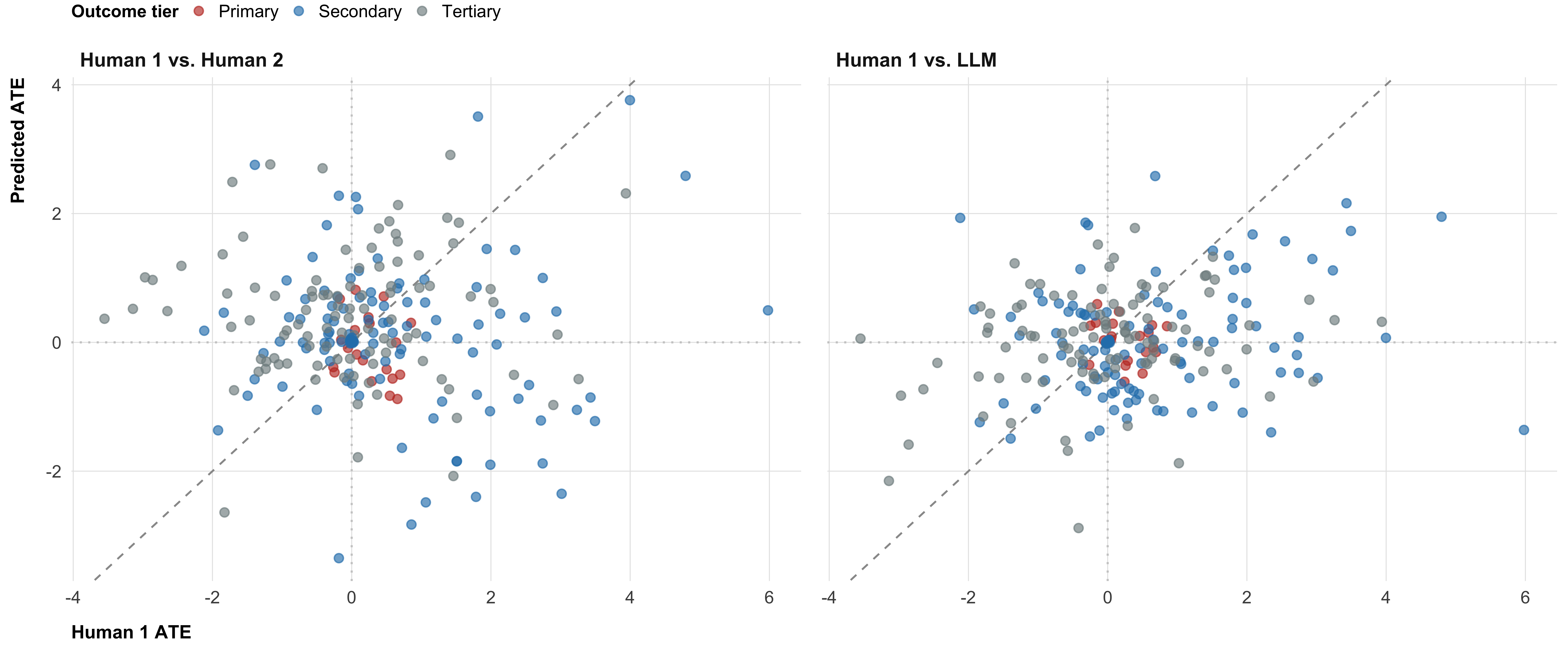
@fig-rq1-pooled shows all `r nrow(pooled_ates)` estimate pairs — one per intervention × outcome combination — colored by outcome tier. Points above the diagonal indicate clone overestimation; points below indicate underestimation.
@tbl-rq1 includes a pooled summary row at the top, followed by per-outcome rows grouped by tier. RMSE is left blank for the pooled row because it is not comparable across outcomes on different scales; all other metrics are scale-invariant. Both comparison pairs (Human 1 vs. LLM and Human 1 vs. Human 2) are reported side by side; the Human 2 columns serve as a human-human ceiling for interpreting LLM performance.
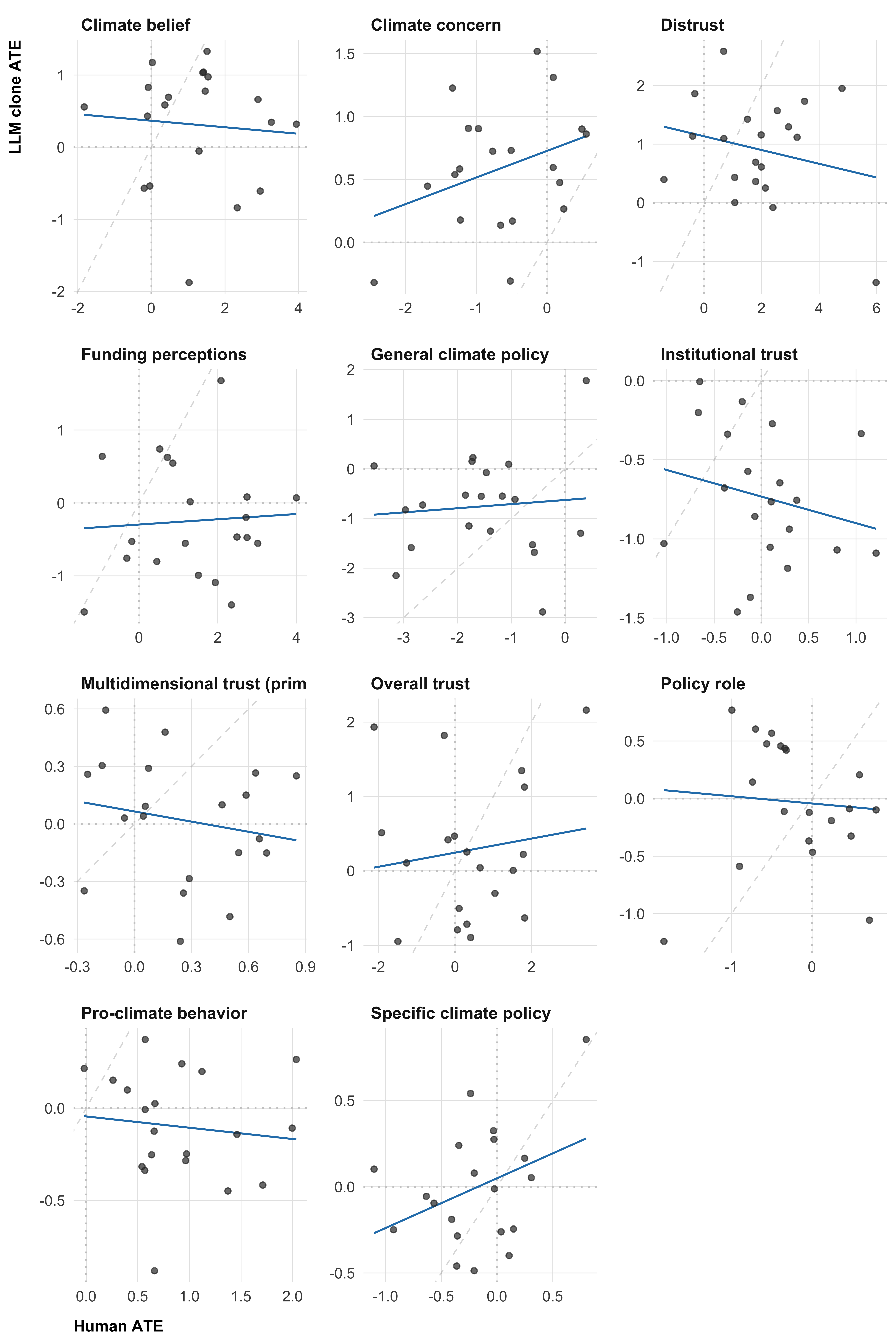
@tbl-rq1-calibration shows calibration regression results for both comparisons (Human 1 vs. LLM and Human 1 vs. Human 2). @fig-rq1-all shows the per-outcome scatter for Human 1 vs. LLM only.
```{r}
#| label: fig-rq1-pooled
#| fig-cap: "ATEs pooled across all outcomes for both comparisons. Left panel: Human 1 vs. LLM clones. Right panel: Human 1 vs. Human 2 (baseline ceiling). Each point is one intervention × outcome pair (N = 240 per panel). The dashed line is perfect agreement; dotted lines mark zero. Color indicates outcome tier."
#| fig-width: 12
tier_colors <- c("Primary" = "#C0392B", "Secondary" = "#2980B9", "Tertiary" = "#7F8C8D")

bind_rows(
  pooled_ates    |> mutate(estimate_pred = estimate_l,  comparison = "Human 1 vs. LLM"),
  pooled_ates_h2 |> mutate(estimate_pred = estimate_h2, comparison = "Human 1 vs. Human 2")
) |>
  ggplot(aes(x = estimate_h, y = estimate_pred, color = tier)) +
  geom_abline(slope = 1, intercept = 0, linetype = "dashed",
              color = "grey60", linewidth = 0.5) +
  geom_hline(yintercept = 0, linetype = "dotted", color = "grey80") +
  geom_vline(xintercept = 0, linetype = "dotted", color = "grey80") +
  geom_point(size = 2, alpha = 0.65) +
  scale_color_manual(values = tier_colors, name = "Outcome tier") +
  facet_wrap(~ comparison, ncol = 2) +
  labs(x = "Human 1 ATE", y = "Predicted ATE") +
  plot_theme +
  theme(legend.position = "top")
```
```{r}
#| label: tbl-rq1
#| tbl-cap: "RQ1 comparison metrics. The 'All outcomes' row pools all estimate pairs across outcomes; RMSE (—) is omitted because outcomes differ in scale. Per-outcome rows each have N = 20 intervention pairs. Left columns: Human 1 vs. LLM clone; right columns: Human 1 vs. Human 2 (baseline ceiling). TOST: % of pairs achieving equivalence (Δ = 50% of human ATE)."
ate_metrics |>
  rename_with(~ paste0(.x, "_llm"),
              .cols = c(spearman_rho, pearson_r, rmse,
                        directional_pct, inferential_pct, tost_pct)) |>
  left_join(
    ate_metrics_h2 |>
      rename_with(~ paste0(.x, "_h2"),
                  .cols = c(spearman_rho, pearson_r, rmse,
                             directional_pct, inferential_pct, tost_pct)) |>
      select(outcome, ends_with("_h2")),
    by = "outcome"
  ) |>
  arrange(match(tier, c("All outcomes", "Primary", "Secondary", "Tertiary")), outcome_label) |>
  select(Tier = tier, Outcome = outcome_label,
         spearman_rho_llm, pearson_r_llm, rmse_llm,
         directional_pct_llm, inferential_pct_llm, tost_pct_llm,
         spearman_rho_h2, pearson_r_h2, rmse_h2,
         directional_pct_h2, inferential_pct_h2, tost_pct_h2) |>
  gt(groupname_col = "Tier") |>
  cols_label(
    spearman_rho_llm    = "Spearman ρ", pearson_r_llm    = "Pearson r", rmse_llm    = "RMSE",
    directional_pct_llm = "Dir. (%)",   inferential_pct_llm = "Infer. (%)", tost_pct_llm = "TOST (%)",
    spearman_rho_h2     = "Spearman ρ", pearson_r_h2     = "Pearson r", rmse_h2     = "RMSE",
    directional_pct_h2  = "Dir. (%)",   inferential_pct_h2  = "Infer. (%)", tost_pct_h2  = "TOST (%)"
  ) |>
  tab_spanner(label = "Human 1 vs. LLM", columns = ends_with("_llm")) |>
  tab_spanner(label = "Human 1 vs. Human 2", columns = ends_with("_h2")) |>
  fmt_number(columns = c(spearman_rho_llm, pearson_r_llm, rmse_llm,
                          spearman_rho_h2,  pearson_r_h2,  rmse_h2), decimals = 3) |>
  sub_missing(columns = c(rmse_llm, rmse_h2), missing_text = "—") |>
  fmt_number(columns = c(directional_pct_llm, inferential_pct_llm, tost_pct_llm,
                          directional_pct_h2,  inferential_pct_h2,  tost_pct_h2), decimals = 1) |>
  tab_style(
    style     = cell_text(weight = "bold"),
    locations = cells_row_groups()
  )
```
```{r}
#| label: tbl-rq1-calibration
#| tbl-cap: "Calibration regression by outcome. α: intercept (systematic bias, with 95% CI). β: slope (proportionality; 1 = perfect, with 95% CI). R²: variance explained. p(β=1): F-test of proportional calibration. Left columns: Human 1 vs. LLM; right columns: Human 1 vs. Human 2 (baseline ceiling)."
calib_metrics |>
  left_join(
    calib_metrics_h2 |>
      select(outcome,
             alpha_h2 = alpha, alpha_lo_h2 = alpha_lo, alpha_hi_h2 = alpha_hi,
             beta_h2  = beta,  beta_lo_h2  = beta_lo,  beta_hi_h2  = beta_hi,
             r_squared_h2 = r_squared, p_beta_1_h2 = p_beta_1),
    by = "outcome"
  ) |>
  arrange(match(tier, c("Primary", "Secondary", "Tertiary")), outcome_label) |>
  mutate(
    beta_ci      = paste0("[", round(beta_lo,     2), ", ", round(beta_hi,     2), "]"),
    alpha_ci     = paste0("[", round(alpha_lo,    2), ", ", round(alpha_hi,    2), "]"),
    beta_ci_h2   = paste0("[", round(beta_lo_h2,  2), ", ", round(beta_hi_h2,  2), "]"),
    alpha_ci_h2  = paste0("[", round(alpha_lo_h2, 2), ", ", round(alpha_hi_h2, 2), "]")
  ) |>
  select(Tier = tier, Outcome = outcome_label,
         alpha, alpha_ci, beta, beta_ci, r_squared, p_beta_1,
         alpha_h2, alpha_ci_h2, beta_h2, beta_ci_h2, r_squared_h2, p_beta_1_h2) |>
  gt(groupname_col = "Tier") |>
  cols_label(
    alpha = "α", alpha_ci = "95% CI (α)", beta = "β", beta_ci = "95% CI (β)",
    r_squared = "R²", p_beta_1 = "p (β=1)",
    alpha_h2 = "α", alpha_ci_h2 = "95% CI (α)", beta_h2 = "β", beta_ci_h2 = "95% CI (β)",
    r_squared_h2 = "R²", p_beta_1_h2 = "p (β=1)"
  ) |>
  tab_spanner(label = "Human 1 vs. LLM",
              columns = c(alpha, alpha_ci, beta, beta_ci, r_squared, p_beta_1)) |>
  tab_spanner(label = "Human 1 vs. Human 2",
              columns = c(alpha_h2, alpha_ci_h2, beta_h2, beta_ci_h2, r_squared_h2, p_beta_1_h2)) |>
  fmt_number(columns = c(alpha, beta, r_squared, alpha_h2, beta_h2, r_squared_h2), decimals = 3) |>
  fmt_number(columns = c(p_beta_1, p_beta_1_h2), decimals = 3) |>
  tab_style(
    style     = cell_text(weight = "bold"),
    locations = cells_row_groups()
  )
```
```{r}
#| label: fig-rq1-all
#| fig-cap: "Human vs. LLM clone ATEs for all continuous outcomes. Each point is one of the 20 interventions; axes are free-scaled across panels. Blue line: OLS regression through the panel's points. Faint dashed line: perfect calibration (slope = 1)."
#| fig-height: 12
map_dfr(outcomes_continuous, function(out) {
  inner_join(
    ate_model_results[[out]]$h |> select(condition, estimate_h = estimate),
    ate_model_results[[out]]$l |> select(condition, estimate_l = estimate),
    by = "condition"
  ) |> mutate(outcome = outcome_label_map[out])
}) |>
  ggplot(aes(x = estimate_h, y = estimate_l)) +
  geom_abline(slope = 1, intercept = 0, linetype = "dashed",
              color = "grey60", linewidth = 0.4, alpha = 0.35) +
  geom_hline(yintercept = 0, linetype = "dotted", color = "grey80") +
  geom_vline(xintercept = 0, linetype = "dotted", color = "grey80") +
  geom_smooth(method = "lm", se = FALSE, color = "#2980B9", linewidth = 0.6) +
  geom_point(size = 1.5, alpha = 0.7, color = "grey20") +
  facet_wrap(~ outcome, scales = "free", ncol = 3) +
  labs(x = "Human ATE", y = "LLM clone ATE") +
  plot_theme
```
### Response Distributions
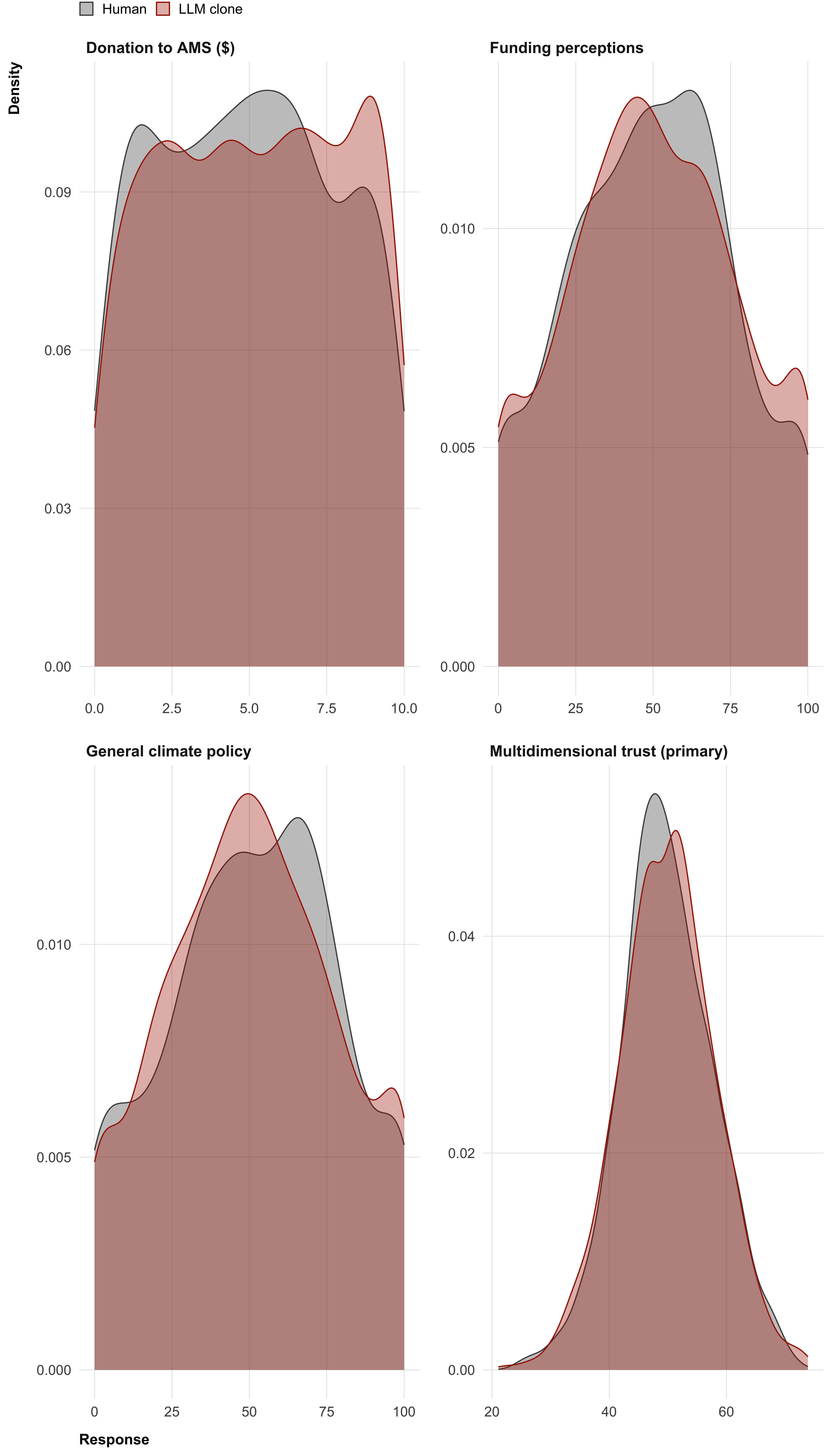
Even if clones match the average treatment effect for each intervention, they may diverge from humans in how responses are distributed: two groups with the same mean can differ in spread, skewness, or tail shape. We ask whether clones reproduce the full response distribution in the control condition — not just the mean — across all continuous outcomes. (`newsletter_signup` is excluded because kernel density estimates are not meaningful for a binary outcome.)
We compare distributions using the same three metrics defined in the methods section, reported in increasing order of strictness. The **variance ratio** (clone / human variance) is the least demanding criterion — it checks only whether spread is calibrated, ignoring shape. The **overlapping coefficient (OVL)** raises the bar to overall shape similarity: it is the proportion of area shared between the two kernel density estimates, equal to 1 when distributions are identical and approaching 0 when they barely overlap. Intuitively, OVL is the overlap area between two smoothed histograms, expressed as a fraction of their total combined area. The **Kolmogorov–Smirnov D-statistic** measures the largest vertical gap between the two cumulative distributions at any point — imagine sliding along the x-axis and tracking how far apart the two curves are; the 'D' statistic is the biggest gap. A value of 0 means the two distributions are indistinguishable everywhere, while larger values flag that at some response value, the two groups diverge sharply.
```{r}
#| label: rq2-compute
control_val <- levels(human_data$condition)[1]

dist_control <- map_dfr(outcomes_illustrative, function(out) {
  compare_distributions(human_data_1, llm_data, out, control_val) |>
    mutate(outcome = out)
}) |>
  mutate(
    tier = case_when(
      outcome == outcomes_primary     ~ "Primary",
      outcome %in% outcomes_secondary ~ "Secondary",
      TRUE                            ~ "Tertiary"
    ),
    outcome_label = outcome_label_map[outcome]
  )

# Human 1 vs. Human 2 baseline ceiling for distribution comparison
dist_control_h2 <- map_dfr(outcomes_illustrative, function(out) {
  compare_distributions(human_data_1, human_data_2, out, control_val) |>
    mutate(outcome = out)
}) |>
  mutate(
    tier = case_when(
      outcome == outcomes_primary     ~ "Primary",
      outcome %in% outcomes_secondary ~ "Secondary",
      TRUE                            ~ "Tertiary"
    ),
    outcome_label = outcome_label_map[outcome]
  )
```
```{r}
#| label: fig-rq2-densities
#| fig-cap: "Response distributions in the control condition, by outcome. Human participants shown in dark grey, LLM clones in orange. Each panel covers the full range of that outcome's scale."
#| fig-height: 14
source_colors <- c("Human" = "grey30", "LLM clone" = met.brewer("Juarez", n = 10)[1])

map_dfr(outcomes_illustrative, function(out) {
  bind_rows(
    human_data_1 |> filter(condition == control_val) |>
      select(value = all_of(out)) |>
      mutate(source = "Human",     outcome = outcome_label_map[out]),
    llm_data   |> filter(condition == control_val) |>
      select(value = all_of(out)) |>
      mutate(source = "LLM clone", outcome = outcome_label_map[out])
  )
}) |>
  filter(!is.na(value)) |>
  ggplot(aes(x = value, fill = source, color = source)) +
  geom_density(alpha = 0.35, linewidth = 0.4) +
  scale_fill_manual(values  = source_colors, name = NULL) +
  scale_color_manual(values = source_colors, name = NULL) +
  facet_wrap(~ outcome, scales = "free", ncol = 2) +
  labs(x = "Response", y = "Density") +
  plot_theme +
  theme(legend.position = "top")
```
```{r}
#| label: tbl-rq2
#| tbl-cap: "Response distribution metrics in the control condition, by outcome. OVL: overlapping coefficient (1 = identical). KS D: Kolmogorov–Smirnov D-statistic (0 = identical CDFs). Variance ratio: clone / human variance (1 = equal spread). Left columns: Human 1 vs. LLM; right columns: Human 1 vs. Human 2 (baseline ceiling)."
dist_control |>
  left_join(
    dist_control_h2 |> select(outcome, ovl_h2 = ovl, ks_d_h2 = ks_d, vr_h2 = variance_ratio),
    by = "outcome"
  ) |>
  arrange(match(tier, c("Primary", "Secondary", "Tertiary")), outcome_label) |>
  select(Tier = tier, Outcome = outcome_label,
         ovl, ks_d, variance_ratio, ovl_h2, ks_d_h2, vr_h2) |>
  gt(groupname_col = "Tier") |>
  cols_label(ovl = "OVL", ks_d = "KS D", variance_ratio = "Var. ratio",
             ovl_h2 = "OVL", ks_d_h2 = "KS D", vr_h2 = "Var. ratio") |>
  tab_spanner(label = "Human 1 vs. LLM",       columns = c(ovl, ks_d, variance_ratio)) |>
  tab_spanner(label = "Human 1 vs. Human 2",   columns = c(ovl_h2, ks_d_h2, vr_h2)) |>
  fmt_number(columns = c(ovl, ks_d, variance_ratio, ovl_h2, ks_d_h2, vr_h2), decimals = 3) |>
  tab_style(
    style     = cell_text(weight = "bold"),
    locations = cells_row_groups()
  )
```
## 2. Subgroup Effects
### Heterogeneity in Treatment Effects
Interventions may work differently for different demographic groups — for example, a message about scientific consensus might shift trust more strongly among Republicans than Democrats, or more among younger than older respondents. We ask whether clones reproduce these subgroup differences, or whether they produce a one-size-fits-all response that averages across demographic groups.
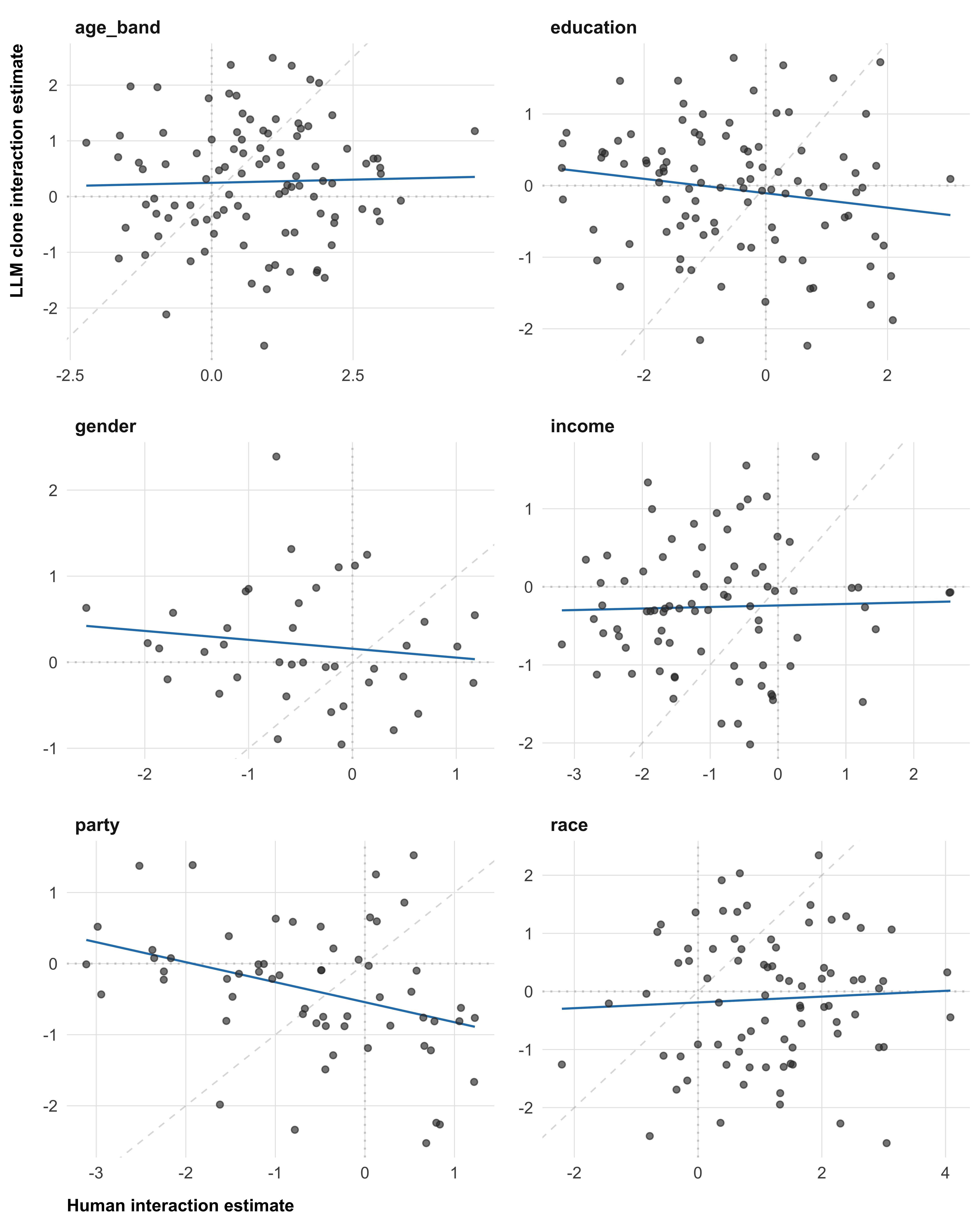
For each of six categorical moderators (gender, age band, race, education, income, and partisan identity), we estimate condition × moderator interactions using `run_moderator_model()` separately on human and clone data for all continuous outcomes. Each interaction term captures how much more (or less) effective a given intervention is for one demographic group compared to the reference group. We compare the full set of interaction estimates between humans and clones using `compare_estimates()`, reporting the six metrics in the same least-to-most-strict order as in Section 1 (directional agreement through TOST equivalence). We first report metrics pooled across all illustrative outcomes and moderators, then break down by outcome.
```{r}
#| label: rq3-models
# Nested: outcome → moderator → model (illustrative subset)
mod_results_all_h <- map(set_names(outcomes_illustrative), function(out) {
  map(set_names(moderators_cat), function(mod) {
    run_moderator_model(human_data_1, outcome = out, moderator = mod)
  })
})
mod_results_all_l <- map(set_names(outcomes_illustrative), function(out) {
  map(set_names(moderators_cat), function(mod) {
    run_moderator_model(llm_data, outcome = out, moderator = mod)
  })
})
mod_results_all_h2 <- map(set_names(outcomes_illustrative), function(out) {
  map(set_names(moderators_cat), function(mod) {
    run_moderator_model(human_data_2, outcome = out, moderator = mod)
  })
})

# Primary-outcome references for the scatter plot below
mod_results_h  <- mod_results_all_h[["trust_multidimensional"]]
mod_results_l  <- mod_results_all_l[["trust_multidimensional"]]
mod_results_h2 <- mod_results_all_h2[["trust_multidimensional"]]
```
```{r}
#| label: rq3-metrics
# All interaction estimate pairs (outcome × moderator × condition × level)
rq3_pooled_interactions <- map_dfr(outcomes_illustrative, function(out) {
  map_dfr(moderators_cat, function(mod) {
    inner_join(
      mod_results_all_h[[out]][[mod]]$interaction_effects |>
        select(condition, moderator_level, estimate_h = estimate),
      mod_results_all_l[[out]][[mod]]$interaction_effects |>
        select(condition, moderator_level, estimate_l = estimate),
      by = c("condition", "moderator_level")
    ) |> mutate(outcome = out, moderator = mod)
  })
})

# Pooled headline (scale-invariant metrics only; RMSE omitted across mixed scales)
rq3_pooled_row <- rq3_pooled_interactions |>
  summarise(
    spearman_rho    = cor(estimate_h, estimate_l, method = "spearman",
                          use = "pairwise.complete.obs"),
    pearson_r       = cor(estimate_h, estimate_l, use = "pairwise.complete.obs"),
    directional_pct = mean(sign(estimate_h) == sign(estimate_l), na.rm = TRUE) * 100
  ) |>
  mutate(outcome_label = "All outcomes", tier = "All outcomes")

# Per-outcome × per-moderator metrics
rq3_metrics_by_outcome <- map_dfr(outcomes_illustrative, function(out) {
  map_dfr(moderators_cat, function(mod) {
    compare_estimates(
      mod_results_all_h[[out]][[mod]]$interaction_effects,
      mod_results_all_l[[out]][[mod]]$interaction_effects,
      join_by = c("condition", "moderator_level")
    ) |> mutate(
      outcome       = out,
      moderator     = mod,
      outcome_label = outcome_label_map[out],
      tier = case_when(
        out == outcomes_primary     ~ "Primary",
        out %in% outcomes_secondary ~ "Secondary",
        TRUE                        ~ "Tertiary"
      )
    )
  })
})

# Human 1 vs. Human 2 baseline ceiling for subgroup effects
rq3_pooled_interactions_h2 <- map_dfr(outcomes_illustrative, function(out) {
  map_dfr(moderators_cat, function(mod) {
    inner_join(
      mod_results_all_h[[out]][[mod]]$interaction_effects |>
        select(condition, moderator_level, estimate_h = estimate),
      mod_results_all_h2[[out]][[mod]]$interaction_effects |>
        select(condition, moderator_level, estimate_h2 = estimate),
      by = c("condition", "moderator_level")
    ) |> mutate(outcome = out, moderator = mod)
  })
})

rq3_pooled_row_h2 <- rq3_pooled_interactions_h2 |>
  summarise(
    spearman_rho    = cor(estimate_h, estimate_h2, method = "spearman",
                          use = "pairwise.complete.obs"),
    pearson_r       = cor(estimate_h, estimate_h2, use = "pairwise.complete.obs"),
    directional_pct = mean(sign(estimate_h) == sign(estimate_h2), na.rm = TRUE) * 100
  ) |>
  mutate(outcome_label = "All outcomes", tier = "All outcomes")

rq3_metrics_by_outcome_h2 <- map_dfr(outcomes_illustrative, function(out) {
  map_dfr(moderators_cat, function(mod) {
    compare_estimates(
      mod_results_all_h[[out]][[mod]]$interaction_effects,
      mod_results_all_h2[[out]][[mod]]$interaction_effects,
      join_by = c("condition", "moderator_level")
    ) |> mutate(
      outcome       = out,
      moderator     = mod,
      outcome_label = outcome_label_map[out],
      tier = case_when(
        out == outcomes_primary     ~ "Primary",
        out %in% outcomes_secondary ~ "Secondary",
        TRUE                        ~ "Tertiary"
      )
    )
  })
})
```
Pooled across all outcomes and moderators, Human 1 vs. LLM: Spearman ρ = `r round(rq3_pooled_row$spearman_rho, 3)`, Pearson r = `r round(rq3_pooled_row$pearson_r, 3)`, directional agreement = `r round(rq3_pooled_row$directional_pct, 1)`%. Human 1 vs. Human 2 (baseline ceiling): Spearman ρ = `r round(rq3_pooled_row_h2$spearman_rho, 3)`, Pearson r = `r round(rq3_pooled_row_h2$pearson_r, 3)`, directional agreement = `r round(rq3_pooled_row_h2$directional_pct, 1)`%.
```{r}
#| label: tbl-rq3
#| tbl-cap: "Interaction estimate comparison metrics by outcome and moderator. Outcomes are grouped by tier; rows are moderators. Spearman ρ: rank correlation across all condition × moderator level pairs. RMSE is in outcome units. Left columns: Human 1 vs. LLM; right columns: Human 1 vs. Human 2 (baseline ceiling)."
rq3_metrics_by_outcome |>
  rename_with(~ paste0(.x, "_llm"),
              .cols = c(spearman_rho, pearson_r, rmse,
                        directional_pct, inferential_pct, tost_pct)) |>
  left_join(
    rq3_metrics_by_outcome_h2 |>
      rename_with(~ paste0(.x, "_h2"),
                  .cols = c(spearman_rho, pearson_r, rmse,
                             directional_pct, inferential_pct, tost_pct)) |>
      select(outcome, moderator, ends_with("_h2")),
    by = c("outcome", "moderator")
  ) |>
  arrange(match(tier, c("Primary", "Secondary", "Tertiary")), outcome_label, moderator) |>
  select(Tier = tier, Outcome = outcome_label, Moderator = moderator,
         spearman_rho_llm, pearson_r_llm, rmse_llm,
         directional_pct_llm, inferential_pct_llm, tost_pct_llm,
         spearman_rho_h2, pearson_r_h2, rmse_h2,
         directional_pct_h2, inferential_pct_h2, tost_pct_h2) |>
  gt(groupname_col = "Tier") |>
  cols_label(
    spearman_rho_llm    = "Spearman ρ", pearson_r_llm    = "Pearson r", rmse_llm    = "RMSE",
    directional_pct_llm = "Dir. (%)",   inferential_pct_llm = "Infer. (%)", tost_pct_llm = "TOST (%)",
    spearman_rho_h2     = "Spearman ρ", pearson_r_h2     = "Pearson r", rmse_h2     = "RMSE",
    directional_pct_h2  = "Dir. (%)",   inferential_pct_h2  = "Infer. (%)", tost_pct_h2  = "TOST (%)"
  ) |>
  tab_spanner(label = "Human 1 vs. LLM",     columns = ends_with("_llm")) |>
  tab_spanner(label = "Human 1 vs. Human 2", columns = ends_with("_h2")) |>
  fmt_number(columns = c(spearman_rho_llm, pearson_r_llm, rmse_llm,
                          spearman_rho_h2,  pearson_r_h2,  rmse_h2), decimals = 3) |>
  fmt_number(columns = c(directional_pct_llm, inferential_pct_llm, tost_pct_llm,
                          directional_pct_h2,  inferential_pct_h2,  tost_pct_h2), decimals = 1) |>
  tab_style(
    style     = cell_text(weight = "bold"),
    locations = cells_row_groups()
  )
```
```{r}
#| label: fig-rq3
#| fig-cap: "Human vs. LLM clone condition × moderator interaction estimates for the primary outcome (multidimensional trust), by moderator. Each point is one condition × moderator level combination. Blue line: OLS regression. Faint dashed line: perfect calibration (slope = 1)."
#| fig-height: 10
map_dfr(moderators_cat, function(mod) {
  inner_join(
    mod_results_h[[mod]]$interaction_effects |>
      select(condition, moderator_level, estimate_h = estimate),
    mod_results_l[[mod]]$interaction_effects |>
      select(condition, moderator_level, estimate_l = estimate),
    by = c("condition", "moderator_level")
  ) |> mutate(moderator = mod)
}) |>
  ggplot(aes(x = estimate_h, y = estimate_l)) +
  geom_abline(slope = 1, intercept = 0, linetype = "dashed",
              color = "grey60", linewidth = 0.4, alpha = 0.35) +
  geom_hline(yintercept = 0, linetype = "dotted", color = "grey80") +
  geom_vline(xintercept = 0, linetype = "dotted", color = "grey80") +
  geom_smooth(method = "lm", se = FALSE, color = "#2980B9", linewidth = 0.6) +
  geom_point(size = 1.5, alpha = 0.65, color = "grey20") +
  facet_wrap(~ moderator, scales = "free", ncol = 2) +
  labs(x = "Human interaction estimate", y = "LLM clone interaction estimate") +
  plot_theme
```
### Response Distributions by Subgroup
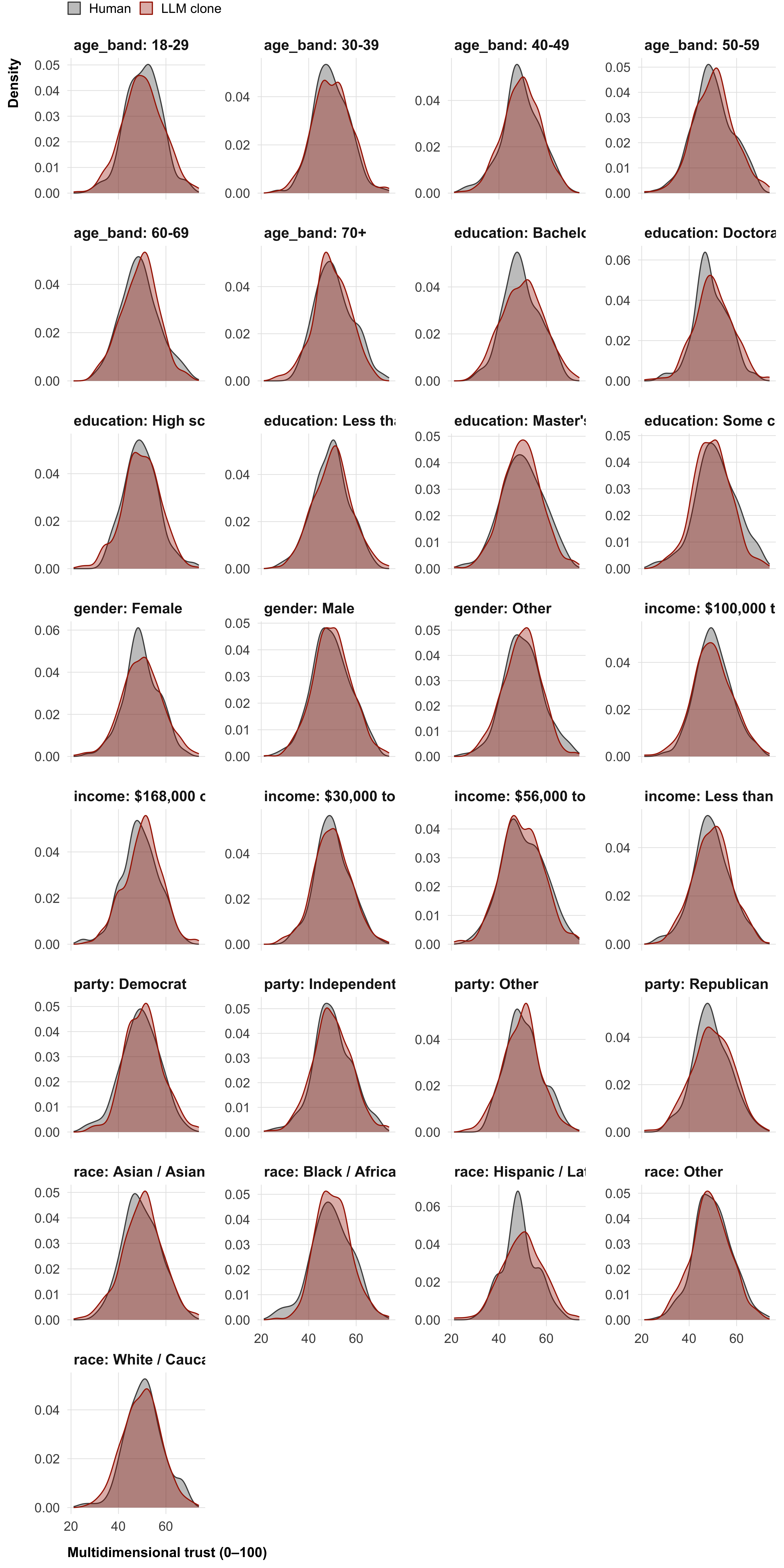
Mirroring the distribution analysis in Section 1, we compare response distributions within each demographic subgroup in the control condition. A clone dataset could reproduce the overall response distribution while having miscalibrated within-group spreads. We use the same OVL, KS D, and variance ratio metrics, in the same increasing order of strictness. These analyses are run separately for all outcomes; the preregistration demonstrates them on the primary outcome (`trust_multidimensional`). Minimum group size of 10 is required for stable kernel density estimation.
```{r}
#| label: rq4c-compute
# For each moderator × level, compare human and clone distributions in control
subgroup_dist <- map_dfr(moderators_cat, function(mod) {
  groups <- levels(human_data[[mod]])
  map_dfr(groups, function(grp) {
    x <- human_data_1 |>
      filter(condition == control_val, .data[[mod]] == grp) |>
      pull(trust_multidimensional) |> na.omit()
    y <- llm_data |>
      filter(condition == control_val, .data[[mod]] == grp) |>
      pull(trust_multidimensional) |> na.omit()
    if (length(x) < 10 | length(y) < 10) return(NULL)
    tibble(moderator = mod, group = grp,
           ovl = compute_ovl(x, y),
           ks_d = suppressWarnings(ks.test(x, y)$statistic),
           variance_ratio = var(y) / var(x))
  })
})

# Human 1 vs. Human 2 baseline ceiling for within-subgroup distributions
subgroup_dist_h2 <- map_dfr(moderators_cat, function(mod) {
  groups <- levels(human_data[[mod]])
  map_dfr(groups, function(grp) {
    x <- human_data_1 |>
      filter(condition == control_val, .data[[mod]] == grp) |>
      pull(trust_multidimensional) |> na.omit()
    y <- human_data_2 |>
      filter(condition == control_val, .data[[mod]] == grp) |>
      pull(trust_multidimensional) |> na.omit()
    if (length(x) < 10 | length(y) < 10) return(NULL)
    tibble(moderator = mod, group = grp,
           ovl = compute_ovl(x, y),
           ks_d = suppressWarnings(ks.test(x, y)$statistic),
           variance_ratio = var(y) / var(x))
  })
})
```
```{r}
#| label: fig-rq4c-densities
#| fig-cap: "Response distributions within demographic subgroups in the control condition (primary outcome: multidimensional trust). Human participants in dark grey, LLM clones in orange."
#| fig-height: 16
map_dfr(moderators_cat, function(mod) {
  groups <- levels(human_data[[mod]])
  map_dfr(groups, function(grp) {
    bind_rows(
      human_data_1 |> filter(condition == control_val, .data[[mod]] == grp) |>
        select(value = trust_multidimensional) |>
        mutate(source = "Human",     panel = paste0(mod, ": ", grp)),
      llm_data     |> filter(condition == control_val, .data[[mod]] == grp) |>
        select(value = trust_multidimensional) |>
        mutate(source = "LLM clone", panel = paste0(mod, ": ", grp))
    )
  })
}) |>
  filter(!is.na(value)) |>
  ggplot(aes(x = value, fill = source, color = source)) +
  geom_density(alpha = 0.35, linewidth = 0.4) +
  scale_fill_manual(values  = source_colors, name = NULL) +
  scale_color_manual(values = source_colors, name = NULL) +
  facet_wrap(~ panel, scales = "free_y", ncol = 4) +
  labs(x = "Multidimensional trust (0–100)", y = "Density") +
  plot_theme +
  theme(legend.position = "top")
```
```{r}
#| label: tbl-rq4c
#| tbl-cap: "Within-subgroup distribution comparison in the control condition. OVL: overlapping coefficient (1 = identical). KS D: Kolmogorov–Smirnov statistic. Variance ratio: second group / Human 1 variance. Left columns: Human 1 vs. LLM; right columns: Human 1 vs. Human 2 (baseline ceiling)."
subgroup_dist |>
  left_join(
    subgroup_dist_h2 |> select(moderator, group, ovl_h2 = ovl, ks_d_h2 = ks_d, vr_h2 = variance_ratio),
    by = c("moderator", "group")
  ) |>
  arrange(moderator, group) |>
  gt(groupname_col = "moderator") |>
  cols_label(group = "Group",
             ovl = "OVL", ks_d = "KS D", variance_ratio = "Var. ratio",
             ovl_h2 = "OVL", ks_d_h2 = "KS D", vr_h2 = "Var. ratio") |>
  tab_spanner(label = "Human 1 vs. LLM",     columns = c(ovl, ks_d, variance_ratio)) |>
  tab_spanner(label = "Human 1 vs. Human 2", columns = c(ovl_h2, ks_d_h2, vr_h2)) |>
  fmt_number(columns = c(ovl, ks_d, variance_ratio, ovl_h2, ks_d_h2, vr_h2), decimals = 3) |>
  tab_style(style = cell_text(weight = "bold"),
            locations = cells_row_groups())
```
## 3. Demographic Baseline Calibration
Section 2 already provides a partial test of demographic stereotyping: if clones exaggerate heterogeneity in treatment effects across subgroups, that is evidence of over-reliance on demographic cues. But there is a second, orthogonal question namely whether clones get the baseline right: For example, the clones could still assign far too low trust to, say, Republicans or far too high trust to Democats before any treatment is applied. This woud be a distinct failure mode — demographic baseline stereotyping rather than effect stereotyping.
Section 3 tests this directly, using only the control condition. It asks two questions: (a) do clone group means match human group means for each demographic group? and (b) do demographic variables predict clone outcomes too strongly — does the demographic profile explain more variance in clone responses than in human responses, indicating that clones map demographics to outcomes too mechanically? Both analyses are run separately for all outcomes; the preregistration illustrates them with the primary outcome (`trust_multidimensional`).
### Demographic Baseline Calibration
For each moderator, we compute mean outcomes within each demographic group in the control condition separately for humans and clones, then correlate and compare those cell means. High correlation and low RMSE indicate that clones start from the right baseline response level for each demographic type — before any intervention is applied.
```{r}
#| label: rq4a-compute
# Cell-mean comparison in the control condition, one moderator at a time
baseline_cal <- compare_demographic_baselines(
  human_data_1, llm_data,
  outcome    = "trust_multidimensional",
  moderators = moderators_cat
)

# Human 1 vs. Human 2 baseline ceiling for demographic calibration
baseline_cal_h2 <- compare_demographic_baselines(
  human_data_1, human_data_2,
  outcome    = "trust_multidimensional",
  moderators = moderators_cat
)
```
```{r}
#| label: tbl-rq4a
#| tbl-cap: "Demographic baseline calibration. For each moderator, cell means in the control condition are compared. r: Pearson correlation of cell means. RMSE: root mean squared error. N cells: number of demographic groups. Left columns: Human 1 vs. LLM; right columns: Human 1 vs. Human 2 (baseline ceiling)."
baseline_cal |>
  left_join(
    baseline_cal_h2 |> select(moderator, r_h2 = r, rmse_h2 = rmse),
    by = "moderator"
  ) |>
  select(Moderator = moderator, r, RMSE = rmse, `N cells` = n_cells, r_h2, rmse_h2) |>
  gt() |>
  cols_label(r_h2 = "r", rmse_h2 = "RMSE") |>
  tab_spanner(label = "Human 1 vs. LLM",     columns = c(r, RMSE)) |>
  tab_spanner(label = "Human 1 vs. Human 2", columns = c(r_h2, rmse_h2)) |>
  fmt_number(columns = c(r, RMSE, r_h2, rmse_h2), decimals = 3)
```
### Demographic Predictability
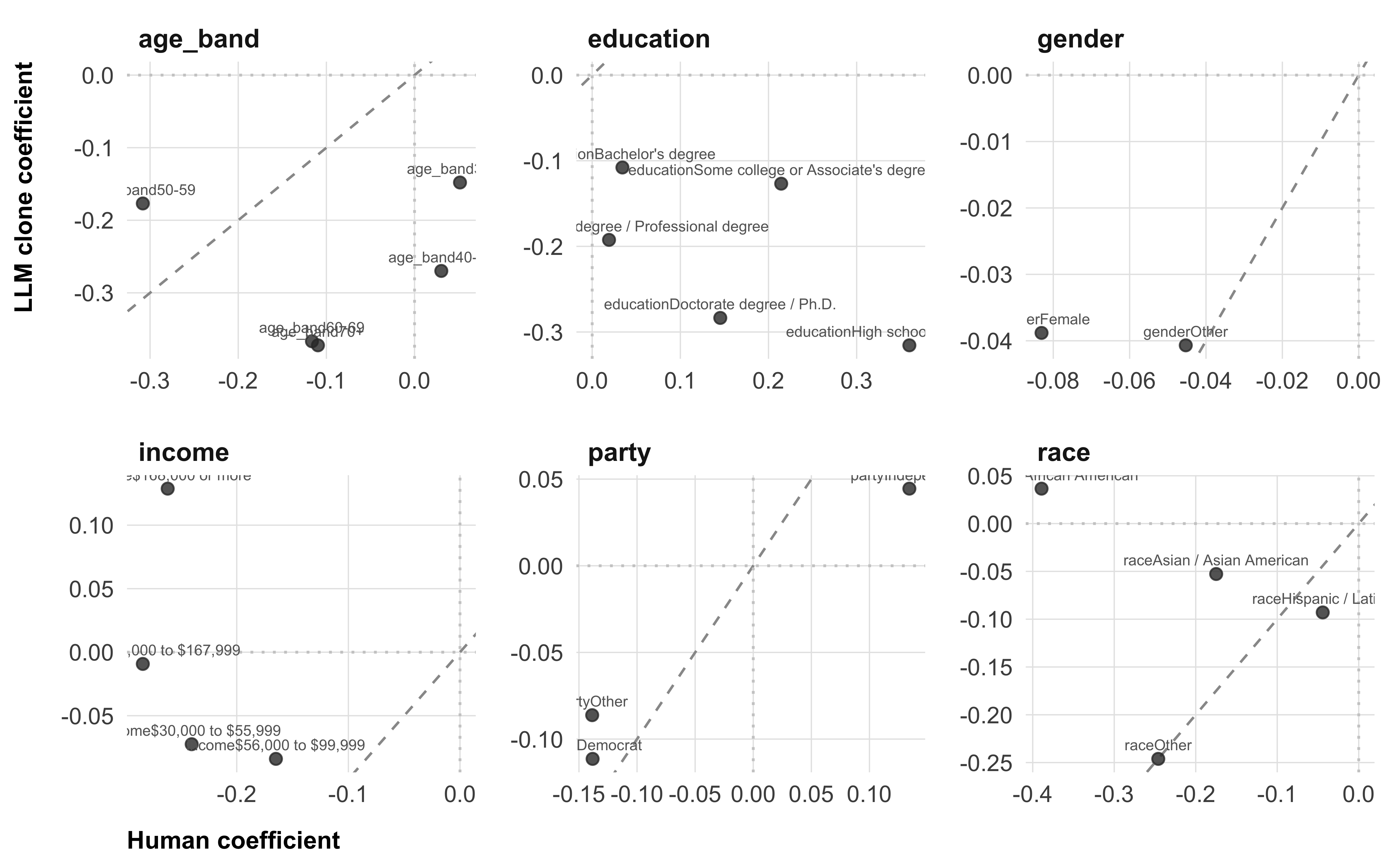
For each of the six demographic moderators we fit a separate OLS regression of the primary outcome on that moderator plus condition fixed effects, on human and clone data independently. Running these regressions separately avoids conflating correlated predictors (race, income, and education are themselves related) and gives a clean per-moderator answer: how much does, say, partisan identity alone explain outcome variance in humans versus clones? If clones over-rely on demographic stereotypes, their R² will be substantially higher than humans' for one or more moderators. We also compare the individual dummy-coded coefficients to identify which groups are over- or underweighted.
```{r}
#| label: rq4b-compute
pred_test <- compare_demographic_predictability(
  human_data_1, llm_data,
  outcome    = "trust_multidimensional",
  predictors = moderators_cat
)

# Human 1 vs. Human 2 baseline ceiling for demographic predictability
pred_test_h2 <- compare_demographic_predictability(
  human_data_1, human_data_2,
  outcome    = "trust_multidimensional",
  predictors = moderators_cat
)
```
```{r}
#| label: tbl-rq4b-rsq
#| tbl-cap: "R² from regressing the primary outcome on each demographic moderator + condition FE. Clone R² >> Human R² signals over-reliance on demographic cues. Human 2 R² provides the baseline ceiling (sampling variation in human predictability)."
pred_test$r_squared |>
  pivot_wider(names_from = source, values_from = r_squared) |>
  left_join(
    pred_test_h2$r_squared |>
      filter(source == "llm") |>
      select(moderator, `Human 2 R²` = r_squared),
    by = "moderator"
  ) |>
  rename(Moderator = moderator, `Human 1 R²` = human, `LLM R²` = llm) |>
  gt() |>
  fmt_number(columns = c(`Human 1 R²`, `LLM R²`, `Human 2 R²`), decimals = 3)
```
```{r}
#| label: fig-rq4b-coefs
#| fig-cap: "Demographic regression coefficients for the primary outcome in humans (x-axis) vs. LLM clones (y-axis), faceted by moderator. Each point is one dummy-coded level. The dashed line marks perfect agreement (slope = 1)."
pred_test$coefficients |>
  ggplot(aes(x = est_h, y = est_l)) +
  geom_abline(slope = 1, intercept = 0, linetype = "dashed",
              color = "grey60", linewidth = 0.5) +
  geom_hline(yintercept = 0, linetype = "dotted", color = "grey80") +
  geom_vline(xintercept = 0, linetype = "dotted", color = "grey80") +
  geom_point(size = 2, alpha = 0.8, color = "grey20") +
  geom_text(aes(label = term), size = 2.2, vjust = -0.8, color = "grey40") +
  facet_wrap(~ moderator, scales = "free") +
  labs(x = "Human coefficient", y = "LLM clone coefficient") +
  plot_theme
```